| < Previous page | Next page > |
Upslope Wood RecruitmentUpslope Wood Recruitment (Debris Flow)
Parameter Description: A fundamentally important characteristic of watersheds is the connectivity of hillslopes to stream channels. Here, connectivity is considered from the perspective of sediment and organic material delivery via mass wasting processes, specifically debris flows. This specific tool addresses the upslope wood recruitment sources (by landslide and debris flow) to stream channels. See also Delivery.
There are several different types of NetMap output that can be used in this analysis: 1) Generic Erosion Potential-Delivery, 2) Shallow Landslide Potential-Delivery, and 3) Debris flow (reach or junctions). Four other types of information that include information on landslide and debris flow sources, in terms of proportions, are: 4) Landslide source proportion, 5) Debris flow traversal, 6) Traversal proportion, and 7) Source traversal proportion. These data layers are located in the Shallow landslide tool (#4) and in the debris flow tool (#5-7). All data layers are grids (rasters) with the exception of debris flow reach and debris flow junctions (reach shape file).
The data layers #1, #2, and 4 through 7 consider delivery to stream channels and an analyst specifies the gradient threshold for wood (or sediment) delivery. The default channel gradient threshold in NetMap datasets is 200% (e.g., all channels). Refer to the Delivery Tool.
Data Type: Line (stream layer) (In Erosion - Debris Flow Tool)
Field Name: P_DF_AVE; Common Name: Debris Flow Susceptibility
Field Name: DF_Junct; Common Name: Debris Flow Susceptibility – Junctions
Data Type: Grid (raster) (In Erosion - Sediment Delivery Tool)
Grid name: SrcProp_ID; Common Name: Common name: Source landslide proportions grid
Grid name: trav_ID (trav); Common Name: Debris flow traversal (the probability of debris flows traversing channel grid cells)
Grid name: travProp_basinID; Common Name: Debris flow traversal proportion grid
Grid name: proportions_basinID; Common Name: SrcTrav_proportion and travprop combined
Units: Refer to specific tools and output
NetMap Module/Tool: Vegetation/Fire/Climate/Riparian Management - Upslope Wood Recruitment
Background:
In Brief:
SrcProp
The proportion of area that encompasses landslide initiation points (GEP based shallow landslide grid cells), 0 – 25% = the highest 25% of landslide initiation points starting with the most unstable, 25-50%, the next quartile etc. all four quartiles = 100% of all of the landslide risk; for example, using the first three quartiles will yield a map that captures 75% of all landslide risk – could also make the legend in terms of tens of percent, or in the GUI could have the ability of a user to select the proportion of risk targeted, top 70%, top 80%, top 90% etc. Note the gradient delivery threshold does NOT apply to this output Trav
this is the probability of debris flow traversal in individual cells, and it is based on a GIVEN gradient threshold for that traversal – relatively low values 0.001 etc. For example, the amount of traversal with a delivery of 0.2 will be a lot higher than with a delivery of 0.02, - we are talking about the length of debris flow track (and probability) than can get into 2% streams and less; there are many more debris flows that can deliver to channels less than or equal to 20% TravProp
This is similar to Src_prop, it takes Trav and assess it in terms of the cumulative distribution, starting at maximum trav values (debris flow traversal values) – this should go into the Erosion Module as well as the Riparian Management module. Trav proportion also has the same gradient threshold option Proportions
This combines Src_prop and Trav_prop into a combined distribution from high to low of landslide source areas and debris flow runout. Additional Detail
Use the srcprop, travprop, and proportions rasters for identifying potential debris-flow source areas and corridors that may serve as sources of large wood for recruitment to the channels of interest. The srcprop identifies debris flow source areas in terms of the proportion of expected future debris-flow initiation sites that generate debris flows that travel to the selected channel reaches. These rasters are a bit tricky to interpret, so please continue reading. Source areas are first characterized in terms of the density of debris-flow initiation sites. "Density" here indicates the number of sites per unit area and was determined as a function of topographic attributes and forest cover using data collected by ODF and Siuslaw National Forest after the 1996 storms. We are able to characterize landslide density in terms of topography and forest cover, because we observe more landslides in areas with steep, convergent topography and fewer landslides in areas with less steep, less convergent topography. Likewise, we observed more landslides in areas with young forest stands (e.g., < 10 yrs) than in areas with older forests. We can translate these observations to maps of expected relative landslide density which show how landslide density is observed to vary across the landscape, from high to low values. To create a "relative" density, we divide all values by the highest observed density, so relative values vary from 1 to zero. This allows us to compare landslide density maps from areas with different data sources.
Because landslide density indicates the number of landslides per unit area, we can calculate the number of landslides observed in any area by integrating the landslide density values over area. In a GIS context, that means we sum pixel values. If we have 100 pixels with landslide density values of 0.01, we expect to find one landslide somewhere within the area covered by those 100 pixels. We take all the pixels with landslide density greater than zero, and starting with the pixels with the largest values, sum the values and assign the sum to the pixel. This allows us to interpret landslide density in terms of the total number of landslides occurring within areas having a density value greater than or equal to some value. We run through all the pixels in the raster, and then divide the sums by the total number of landslides. Each pixel then has a value that indicates the proportion of all landslide initiation sites encompassed with pixels having that value or less. These are written to the srcprop raster. So if you select all pixels in srcprop with a value greater than zero but less than 0.10, it will show the areas with the highest landslide density where we expect to see 10% of all future landslides initiated (that then traveled to the selected channels) over the area mapped. This provides a way to quantitatively map landslide susceptibility and potential for landslide delivery of wood to channels. If you want to identify those landslide initiation sites that will account for 50% of future landslides that delivery wood to the selected channels, you would select all pixels in scrprop with values greater than zero but less than 0.5. If you wanted to identify those sites that will account for 80% of future landslides that delivery wood to the selected channels, you would select all pixels in scrprop with values greater than zero but less than 0.8.
Srcprop is looking only at landslide initiation sites - the source areas for debris flows, and it is looking only at initiation sites for landslides that can actually travel to the selected channels. That's the source-area part of the story. Much of the wood in debris-flow deposits is not from the initiation site, however, but was picked up along the way through scouring headwater streams. The second part of the story, therefore, is to identify debris-flow corridors where both standing and fallen trees can be picked up by a debris flow and carried to a channel of interest. That's what travprop is intended to show. To do this, we developed a statistical model that describes the probability for a debris flow to travel from its initiation point to locations downslope, again using data collected by ODF after the 1996 storms. With this model, we can identify which landslide initiation sites can actually trigger debris flows that can carry wood to the selected channels. By combining it with the model described above for estimating the probable locations of landslide initiation sites, we can describe the observed debris-flow-track density (length of debris-flow track per unit area) as a function of the number of upslope initiation points, the probability of initiation from each upslope point, and of topographic and forest-cover attributes along the downslope flow path from each initiation site. We can create a map of debris-flow-track density. If we integrate this density over area (or within a GIS, sum pixel values) we get the observed (or expected) debris-flow track length within any area. When we divide by total debris-flow-track length, we get the proportion of total debris-flow-track length observed (or expected) within any area. Then we can sort pixels by debris-flow-track-length density and sum values, from high to low, to get the total debris-flow-track length associated with density values greater than or equal to the value of the pixel. We divide these values by the total length over all, so that pixel values represent the proportion of observed (or expected) debris-flow track length.
So to identify the most frequently traversed debris-flow corridors that contain 10% of the total expected debris-flow track length within the mapped area, you use the travprop raster and select pixels with values greater than zero and less than or equal to 0.10. To identify those corridors that contain 50% of the total expected track length, choose pixels with values greater than zero and less than or equal to 0.50. In creating the travprop raster, we added a buffer (although I don't recall how large the buffer is - it will show up in the log files for the travprop raster) to account for the uncertainty in translating from DEM locations to on-the-ground locations. The proportions raster merges the srcprop and travprop rasters to show where buffers would be placed to protect a given proportion of both debris-flow source areas and travel corridors.
Examples follow:
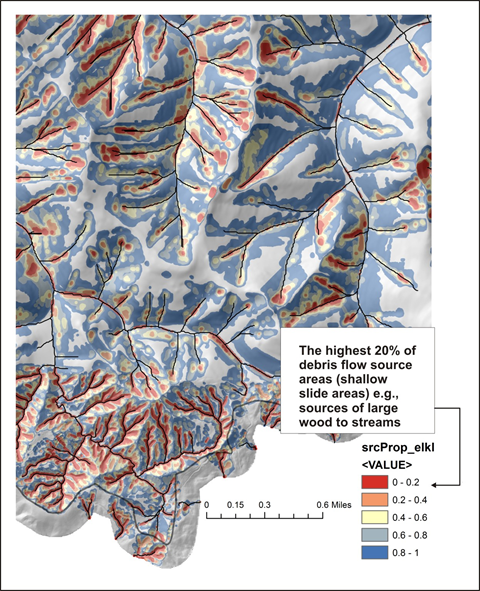 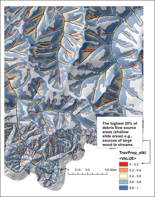 Left panel: The NetMap attribute SrcProp that can be used to identify upslope areas that can contribute large wood to streams. Defined as the proportion of area that encompasses landslide initiation points (GEP based shallow landslide grid cells), 0 – 0.2 = the highest 20% of landslide initiation points starting with the most unstable, 20-40%, the next quartile etc. all four quartiles = 100% of all the landslide risk. Right panel: Trav_Prop, a NetMap attribute that can be used to identify upslope zones of large wood recruitment, in terms of cumulative probability of debris flow traversal in individual cells, and it is based on a gradient threshold for that traversal; default value is >=0.04. For example, the amount of traversal with a delivery of 0.2 will be higher than with a delivery of 0.02.
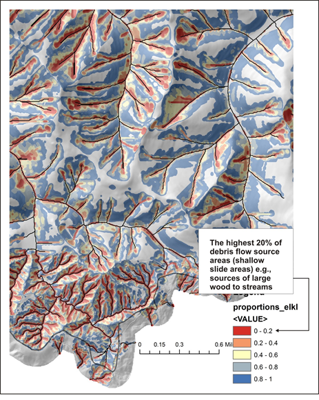 Figure: Proportions, a NetMap attribute that can be used to identify upslope zones of large wood recruitment, in terms of cumulative probability of 1) shallow landslide potential and debris flow runout in individual cells, and it is based on a gradient threshold for that traversal; default value is >=0.04. For example, the amount of traversal with a delivery of 0.2 will be higher than with a delivery of 0.02. This attribute combines the two figures above. More Info:
Debris flows are typically triggered in unchanneled and steep areas in watersheds and they traverse headwater streams and deposit sediment and woody debris (including who trees) into fish bearing streams. Debris flows occur in old growth forests during intense rainstorms (Figures 1 and 2), following fires (Figure 3) and following timber harvest and road construction (Figure 4). In all of these environments, debris flows can represent a risk to aquatic resources. Negative effects of debris flows may include immediate burial of existing habitat and direct mortality of aquatic biota; increased fine sediment in gravels onsite and downstream that suffocates fish eggs in gravel (Everest et al. 1987; Scrivener and Brownlee 1989); increased bedload transport and lateral channel movement due to heightened sediment supply that scours fish eggs; and loss of pools that reduces rearing habitat (Frissel and Nawa, 1992; Hogan et al. 1998).
Landslides and debris flows may also have a positive effect on aquatic ecosystems. Beneficial effects of debris flows on aquatic systems include formation of ponds that become occupied by fish and beaver (Everest and Meehan 1981); release of nutrients due to buried organics in anaerobic environments (Sedell and Dahm 1984); deposition of woody debris that creates sediment wedges and forms pools (Hogan et al. 1998; Reeves et al. 2006; Bigelow et al. 2007); deposition of boulders that trap sediments and create complex habitats (Reeves et al. 1995); formation of wider valley floors that contain larger floodplains (Grant and Swanson 1995); and increased biological productivity (Roghair et al. 2002). Spates of debris flows may also contribute to watershed-scale habitat diversity, including in riparian forests (Nierenberg and Hibbs 2000; Nakamura and Swanson 2002; Bigelow et al. 2007).
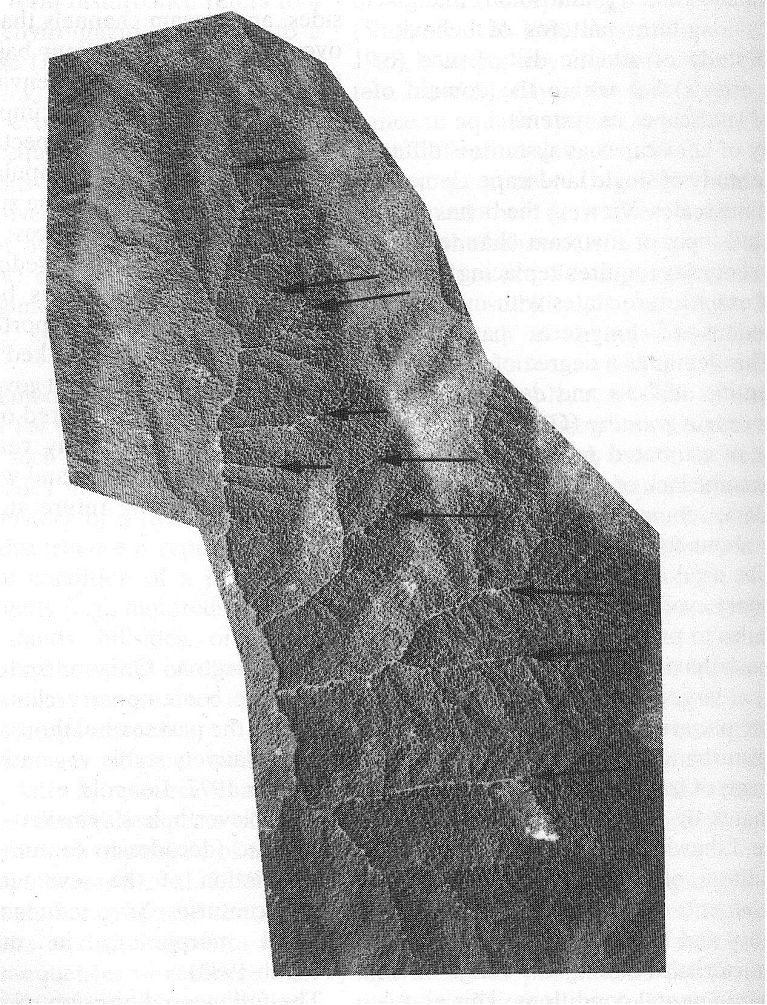 Figure 1. A 1939 aerial photograph of an old growth forest in the Olympic Peninsula, Washington, shows how a very large storm (1934) triggered numerous debris flows at the heads of first order streams. Most of the debris flows traversed through headwater (first and second order) streams and deposits sediment and wood in higher order fish bearing streams (from Benda et al. 1998). This type of watershed has high connectivity.
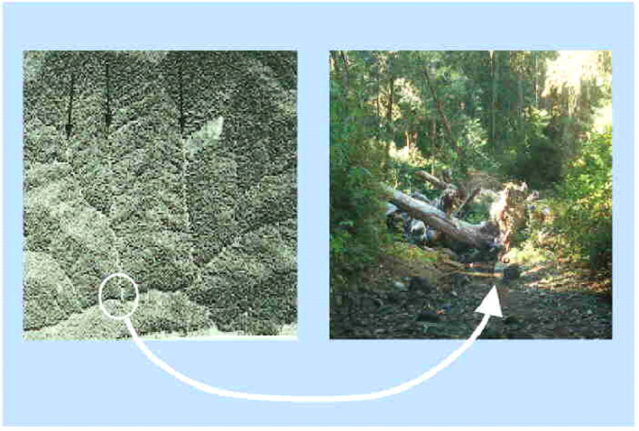 Figure 2. In some landscapes debris flows in headwater, first- and second-order channels are important sources of wood to larger, fish bearing channels. Although some proportion of debris flows deposit upstream of tributary junctions, many scour and travel until they reach a sharp-angled tributary junctions at larger fish-bearing streams, even in wilderness conditions as shown here in the Olympic Peninsula, WA (left panel). NetMap contains a tool for evaluating the importance of debris flows as a wood recruitment agent in larger, fish-bearing channels. An example from an old growth forest in the Oregon Coast Range (right panel) shows accumulations of large logs that was deposited by a debris flow at the mouth of a second order streams (right panel); see also Bigelow et al. 2007.
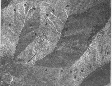 Figure 3. Stand replacing fires in the Tillamook basin, Oregon Coast Range, in conjunction with large rainstorms triggered numerous shallow landslides and debris flows (from Benda and Dunne 1997a). Wildfires can increase the connectivity between hillslopes and streams.
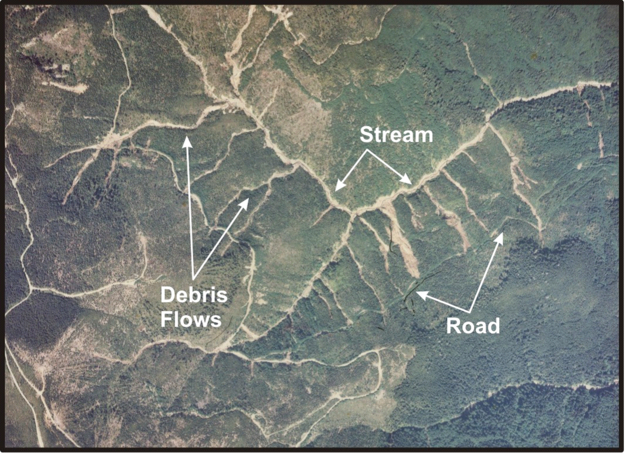 Figure 4. An extreme example of poor road building, widespread clearcutting and a large storm yielding numerous debris flows that deposited sediment and organic material into fish bearing streams (in northwest Washington). This highly dissected landscape has great potential for very high connectivity, particularly following the destabilizing effects of road construction and timber harvest.
NetMap contains a tool for predicting debris flows and their potential ecological impacts on streams and rivers.
In this model, there are two types of source areas for large wood to fish bearing streams and rivers:
1. hillslope areas that trigger debris flows that travel to fish-bearing streams, and
2. steep headwater channels that are traversed by debris flows prior to depositing in lower gradient, fish bearing channels.
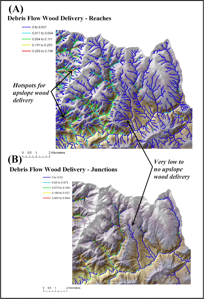 Figure 5. The wood delivery potential of debris flows to lower gradient channels is predicted for a portion of the Clatskanie River basin. (A) Predictions for the entire stream network. (B) Predictions at junctions only in mainstem channels – mainstem junction values are the same as the value in the lowest segment of intersecting headwater tributaries; if more than two tributaries intersect a given mainstem segment, the highest probability value is recorded.
More Background:
There are a variety of models available to predict shallow landslides, primarily for humid mountain landscapes (Sidle 1987, Montgomery and Dietrich 1994, Pack et al. 1998). Most models require information on hillslope topography, including gradients and some measure of convergence. Topographic information provided by 1:24,000 scale mapping does not resolve all topographic features pertinent to landslide locations (Benda and Dunne 1997). For instance, the landslide model does not account for small streamside failures (often referred to as inner gorge landslides) because of the inability of 10-m DEMs to resolve low relief landforms. Mapped landslide potential may also not resolve all small convergent areas, important to project level site-specific assessments. However, mapped landslide potential resolves topographic controls over larger areas, such as the relative risk between different first-order basins or between larger watersheds.
Slope gradient provides a basic topographic index for which relative landslide densities can be calculated. Other options include the SHALSTAB model [Dietrich and Montgomery, 1998] and the product of slope and local drainage area (that within a 10-m radius). For this project, we used the later, because it provided the greatest resolution of mapped landslide locations, in that it requires the smallest proportion of the study-site area to encompass a given proportion of all mapped landslide initiation points (Miller and Burnett 2007a).
The landslide density model allows for a somewhat finer grained resolution of landslide potential compared to Generic Erosion Potential (GEP) (Figure 5). Although it also focuses on slope gradient and convergence, landslide density values reflect a topographic weighting that is calculated according to a comprehensive shallow landslide inventory. The landslide density predictions (#/km2) pertain specifically to the magnitude of the storm represented in the landslide inventory. For instance, the landslide density is what would be expected during another identical storm. Since there are many storms that can trigger landslides, we recommend that landslide density be used as a relative index (from high to low), although the specific numerical values for landslide density are available in the legend editor and can be displayed if desired. Specific landslide density values to create fixed categories of landslide potential (reflected in the different color codes) can be created to allow comparison across diverse watersheds.
The example mapping of landslide density in the northeastern portion of the Wilson and Trinity River watersheds reveals significant spatial variability. Such maps can be used as a screen by field foresters and geotechnical specialists. Use of generic erosion potential and landslide density predictions can be used to learn how to identify landslide prone areas in the field and from aerial photography.
Landslide Initiation
The first component, hillslope sources of debris flows, is based on a landslide model by Burnett and Miller (2007), described elsewhere in NetMap’s Technical Help. To summarize, the parameter of ‘landslide density’ in the model is the number of landslides per unit land area (e.g., 1.2 landslides per km2, or 536 m2 landslide area per km2). Landslides tend to occur in certain types of locations. For example, translational failure of shallow soil layers – the type of landslide that tends to trigger debris flows in the Pacific Northwest – tend to occur on steep slopes (e.g., Sidle and Ochiai 2006). Such landslides do not occur in low-gradient terrain, and the number of landslides per unit area (landslide density) varies empirically with slope steepness (e.g., hillslopes with gradients between 50% and 60% may have 0.4 landslides per km2, whereas slopes with gradients between 60% and 70% may have 0.8 landslides per km2).
Rather than slope gradient alone, a gradient weighted by a measure of topographic convergence, is used to better resolve landslide terrain than slope gradient alone (in that a larger proportion of the landslides are included in a smaller proportion of the area) (Miller and Burnett 2007), based on an approach proposed by Montgomery and Dietrich (1994). An example of predicted landslide density is shown in Figure 8.
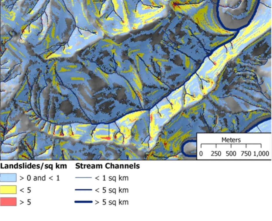 Figure 8. Landslide density is predicted for Lake Creek in the Oregon Coast Range. Extensive areas have a low predicted density with large values confined to steep slopes and bedrock hollows.
To obtain a value more readily interpreted in terms of relative landslide susceptibility, landslide density is converted to proportion of landslides, area weighted. Using slope-classes, the areas in specific slope steepness-area class are multiplied by landslide density. For example, suppose we have mapped 100 landslides within a 100 km2 watershed, and our DEM-derived slopes show that areas with gradients between 60% and 70% cover 5 km2, and 25 of the mapped landslides lie in those areas. Then those slopes contain 25% of the mapped landslides, cover 5% of the watershed area, and have a landslide density of 4 landslides per km2. Moreover, to assess landslide potential, we assume that in the future, 25% of the landslides that occur in the watershed will, averaged over time, occur on those slopes. We perform the same exercise for every slope class. Each class then has a known landslide density, contains a known proportion of the landslides, and covers a known proportion of the watershed area.
Classes are ordered in terms of decreasing landslide density, the number of landslides in each class (going from least stable – highest density – to most stable – lowest density) are summed to arrive a cumulative total, and then divide by the total to get a proportion. This provides a means to delineate areas in terms of an easily interpreted measure of landslide potential. If we want to delineate the smallest area that includes 25% of all mapped landslides, we’d include all areas with a value greater than zero and less-than-or-equal to 0.25; if we want the smallest area that includes 85% of all landslides, we’d include areas with values greater than zero and less-than-or-equal to 0.85 (fieldname = initProp, for initiation proportion) (Figure 9). The patterns are similar as those shown for landslide density in Figure 8, but in terms of the proportion of (expected) landslides included in any delineated area.
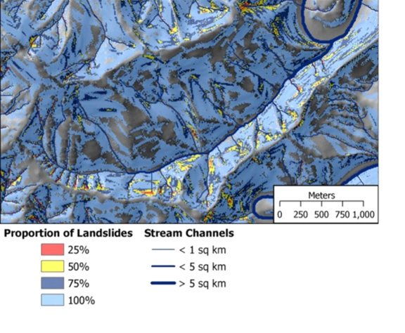 Figure 9. Shown are the areas encompassing a given proportion of expected landslides, starting with the least stable areas (in red). For example red zones cover 25% of the most unstable areas; red plus yellow cover 50% (including 25% of the next highest unstable areas); red, yellow, dark blue and light blue cover all expected landslide terrain. This illustrates the spatially variable nature of hillslope-channel connectivity with respect to mass wasting.
Connectivity or Delivery Potential
The next step in the model is to determine to what extent debris flows, triggered by shallow failures, can move downstream and enter large, fish bearing channels. A great many landslides never directly reach lower gradient (fish bearing) channels. Many landslides are small and don’t travel far (low connectivity); they do not carry wood to fish-bearing streams. Two debris flows initiating from the same shallow landslide location (perhaps separated in time by several centuries) will not necessarily travel the same distance. One may go a short distance, the other very far, depending on a variety of factors that we cannot quantify (e.g., how much material was stored in the debris-flow track, how large the initiating landslide was, how intense the triggering rainstorm was, etc.).
Our approach requires weighting each landslide initiation site by the probability that a debris flow triggered from that site travels to a channel of interest. To do that, we use the second empirical model (Miller and Burnett 2008). SThat model, as with the landslide model described above, uses a population of observed events as an indicator of future events. A set of mapped debris-flow tracks is used to quantify the influence of different landscape attributes – that can be measured using GIS data – on debris-flow-runout extent. Topographic attributes are chosen that are important controls on debris-flow behavior including runout track gradient and confinement, and attributes of channel junctions along the track (junction angle, gradient and confinement of the receiving channel). For additional detals, see Miller and Burnett 2008.
Based on the empirical database of mapped debris flows in the Oregon Coast Range (Robison, Mills et al. 1999), probabilities of debris flow scour or deposition were estimated using attributes obtained from the DEM (local gradient, confinement, etc.). Each point along each mapped track is characterized in terms of the cumulative upstream length of scour and deposition and the ratio of these lengths (length of deposition divided by length of scour) is calculated at the point where the debris flow stopped. For any particular value of the ratio, we can then see what proportion of the debris flows had a value that was larger at their terminus and what proportion had a value that was smaller. These proportions are used to estimate the probability. For example, along any potential debris-flow track we can calculate the ratio at all points. If, in our data, 20 out of 100 debris flows had ratio values less than 0.5 at their terminus, then we expect that, along any potential debris-flow track, there is a 20% chance that a debris flow traversing that track will stop upslope of that point (where the ratio of deposit to scour length is 0.5) and an 80% chance that it will stop downslope of that point.
From any potential debris-flow-initiation point, the flow path downslope, DEM-cell-by-DEM-cell, is used to calculate a probability (based on the proportions described above) that a debris flow continues past each cell along the way. We do this for every potential debris-flow-initiation site (every DEM cell with an estimated landslide density greater than zero from the previous model, e.g., Figure 8) and follow the runout path until it hits a channel of interest, or goes to zero. In this way, for every DEM cell, we can estimate the probability that a debris flow triggered from the cell travels to a point of interest (e.g., a fish-bearing stream) (Figure 10).
 Figure 10. The upper map shows the predicted connectivity or the delivery potential of shallow landslides and debris flows (probability) for all streams in the Lake Creek tributary to the Alsea River in Coastal Oregon. The lower map shows the probability for delivery to a channel with gradient less than 7% (to approximate the portion of the channel network used by anadromous fish).
Landslide density (Figure 8) and probability for delivery (Figure 10) together provide a means to assess landslide potential from a stream-channel perspective. If we multiply the landslide density for each DEM cell by the probability for delivery, we get landslide density in terms of the number of landslides that deliver material to streams of interest (of a particular gradient threshold). We then use those values to translate landslide density to proportion of landslides, in this case, proportion of all landslides that deliver material to streams (Figure 11).
 Figure 11. The predicted landslide density for each DEM cell is multiplied by the probability for delivery thereby creating a landslide density in terms of the number of landslides that deliver material to streams of interest (of a particular gradient threshold). Those values are translated into the proportion of all landslides that deliver material to streams.
The steps are as follows: use the initiation model (Figure 8, and see Shallow Landslide in Technical Help) to create a raster file of landslide density, the runout model to create a raster file of delivery probabilities (Figure 10), multiply the two to get a raster (grid) of delivery-weighted landslide density, and use this to generate the proportion-of-sources raster file. To reduce data-file sizes, values are aggregated to 5% bins and exported to a polygon shapefile, which is then used to generate maps to delineate source areas in terms of the proportion of debris flows that deliver, ranked from least to most stable.
Imagine standing in a low-order channels prone to debris flows. The contributing area to this point may contain many potential initiation sites, each one of which has some probability of generating a debris flow that will traverse the point you are standing, pick up the down wood buried beneath your feet, and continue downslope to a fish-bearing stream. We are interested in the likelihood that any of the upslope initiation sites will generate such a debris flow. For this, we interpret the delivery-weighted landslide density from each source DEM cell in terms of the probability that, in our calibration data set, a debris flow was generated from that cell and traveled downslope to a fish-bearing channel. This probability is based solely on the topographic attributes described above. We calculate the probability that such a debris flow didn’t happen, because we can estimate the probability that there were no debris flows from any of the upslope sources by multiplying the probability of non-occurrence over all sources. The probability that a debris flow did occur is then just one minus the probability that none did. We compute this for every DEM cell. So, based on our calibration data set, we estimate the probability for every DEM cell that it was traversed by a debris flow from upslope that continued downslope to a fish-bearing stream. The magnitude of these values is dependent on the number of debris-flow tracks included in our calibration data, so we need a way to normalize.
If we multiply this probability of traversal by flow length through the cell, and sum over all cells, we should get a value equal roughly to the total mapped track length of debris flows that traveled to fish-bearing streams in the calibration data set. We can, therefore, normalize these values in terms of the proportion of expected debris-flow track length. To do this, we rank cells by probability of traversal, multiply each by flow length through the cell, and sum (from largest probability to smallest) to get a cumulative travel length. We divide the cumulative length by the total sum to get a proportion (field name = trav). We calculate a value for every DEM cell. High trav values identify debris-flow corridors to fish-bearing streams.
So far, we’ve been working with raster data. To translate trav values to the vector channel-reach layer, the proportion of the expected debris-flow track length associated with any channel reach is obtained by summing trav values over the cells crossed by that reach. We assume that the calibration data is indicative of future events, so to delineate the smallest portion of the channel network within which a specified proportion of future debris-flow tracks will occur, we flag all channel reaches with an average trav value greater than zero and less than or equal to the proportion of interest. Examples for Lake Creek are shown in Figure 12.
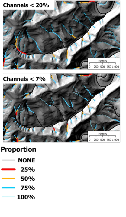 Figure 12. Low order channel, debris flow corridors to fish bearing streams in terms of channels to include in a given proportion of total debris flow track length. Channels of interest are defined in terms of a gradient threshold (<20%, <7%). The proportion is defined over the entire Alsea watershed, of which Lake Creek (shown) is only a small part.
Example Application
The foregoing discussion and modeling can be used to consider hillslope-channel connectivity more generally or the potential for debris flows to couple to fish bearing streams or for considering wood delivery by debris flows. For example, to delineate the smallest area that includes 25% of all landslides that deliver material to fish-bearing streams (based on the model), you would flag all areas with initProp values greater than zero and less than 25%. Note, we are not referring to 25% of the initiation sites (here, the DEM cells identified as potential landslide initiation sites), but to that collection of sites you must include to encompass 25% of the landslides that occur, which will typically entail much less than 25% of the sites. These sites are identified by the topographic attributes characteristic of locations where landslides were mapped in the calibration data set. Likewise, to identify the smallest proportion of the low-order channel network that includes 25% of all debris-flow track length (for those debris flows that traveled to fish-bearing streams), you would flag all channel reaches with trav values greater than zero and less than 0.25. To include all landslide sites that could trigger debris flows that travel to fish-bearing streams, and all low-order channels that could be traversed by a debris flow that travels to a fish-bearing stream, you would flag all areas with non-zero initProp values and all channels with non-zero trav values. The appropriate levels depend on the issue at hand.
Because we do not know a-priori which streams have fish and which don’t, and because some species persist further upstream than others, we provide results for two portions of the channel network:
1. All streams with no down-stream gradient greater than 20%, which corresponds roughly to the upper extent of fish use for all species. The DEMs used for the Oregon Coast Range are interpolated from 40-foot contour lines on 1:24,000-scale USGS topographic maps. To estimate channel gradient, we sum DEM-traced channel length between 40-foot contour-line crossings. Techniques used for tracing channels are described in Clarke et al. (2008).
2. All streams with no down-stream gradient exceeding 7%. This corresponds roughly to the upper extent of anadromous fish use.
The landslide-source areas indicated by initProp can be similar for each case; the proportional values found at any particular site vary between cases, but not as much as the relative change in delivery potential (except where delivery potential to low-gradient streams goes to zero, in which case, initProp also goes to zero). This may seem surprising; in general, the potential for delivery to a low-gradient stream (< 7%) is much lower than the potential for delivery to a high-gradient stream. This is clearly shown in the maps of delivery potential and of delivery-weighted landslide density. One might expect a similar change in initProp. Of the landslides that occur, there may be many that deliver material to the entire channel network, including steep channels, and not so many that travel all the way to low-gradient channels. The total number of landslides involved in each of the two cases is different, but with initProp, we are looking at relative values. The same source areas may be involved in each case, but the number of landslides that deliver to the channels of interest are different.
Likewise, the set of low-order channels identified as debris-flow corridors to fish-bearing streams is similar for both cases. We are dealing only with debris flows that continue downstream to fish-bearing streams. The probability that such a debris flow traverses any point in the channel network depends on the number of upslope debris-flow-initiation sources in the contributing area to that point. As we progress downstream, the contributing area increases and may include additional debris-flow-initiation sources. The potential for traversal by a debris flow (that continues to a fish-bearing stream), therefore, increases downstream (it cannot decrease) at a rate-per-unit-channel length dependent on the location of initiation source areas and the probability for delivery from each. Thus, the reaches with the greatest potential for debris-flow traversal are those at the downstream end of small, steep landslide-prone sub-basins tributary to the fish-bearing network. The downstream extent of these delineated channels is determined by our determination of the upstream extent of the fish-bearing network.
Because we are dealing with relative values, the patterns are dependent on the scale over which the analysis is performed. For example, a large watershed may have some sub-basins where the initProp value never exceeds 0.4. If we were to do the analysis over that sub-basin alone, it would, by definition, have values ranging up to 1.0. For NetMap, we do the analyses over each NetMap data set (roughly the size of a 4th-field hydrologic-unit-code basin).
|