Debris Flow

Debris Flow Susceptibility

Parameter Description: The susceptibility of channels to debris flow movement, scour and deposition, in terms of probability; an empirical model. Predictions include debris flow susceptibility across entire river networks, focusing on headwater streams, and debris flow susceptibilities in mainstem (fish bearing) channels at headwater tributary junctions (e.g., likely areas of debris flows impacts from steeper headwater channels).

There are four component models that address debris flow rish in streams, debris flow risk at tributary confluences (fish eye view), proportion of debris flow risk (0-100%) based on predicted delivery to streams of a specified channel gradient threshold (see Delivery Tool), and combined shallow landslide-debris flow risk proportion (also using a user specified delivery channel gradient threshold).

Important Notice: This erosion model is calibrated for the Oregon Coast Range. Thus when used outside of that landscape, the model should be considered as a screening tool that provides a relative ranking of instability potential(e.g., low - high). Although the model employs universal topographic indicators of debris flow initiation and runout potential increased accuracy and resolution can be obtained when debris flow model is calibrated using local data (georeferenced locations of debris flow initiation and runout). A calibration tool is planned for NetMap in later 2014. Also see Warning about using Slope Stability Models.

Data Type: Line (stream layer)

Field Name: P_DF_AVE; Common Name: Debris Flow Susceptibility

Field Name: DF_Junct; Common Name: Debris Flow Susceptibility – Junctions

Data Type: Grid (raster)

Grid name: trav_ID; Common Name: Debris flow traversal (the probability of debris flows traversing channel grid cells)

Grid name: travprop_basinID; Common Name: Traversal proportion grid

Grid name: proportions_basinID; Common Name: Source Traversal proportion grid

Units: The modeled relative spatial frequency of debris flow scour and deposition (and traversal, neither scour or deposition). For example, all reaches with the same modeled P_DF_AVE value have similar physical characteristics found empirically related to debris-flow occurrence (number of landslide sources, the length, steepness, and confinement of the potential debris-flow tracks leading from those landslide source areas to the reach). The P_DF_AVE value reflects the relative proportion of similar reaches mapped with debris-flow effects. We expect, therefore, out of 1000 reaches with a P_DF_AVE value of 0.02, we should find twice as many with evidence of debris-flow deposition or scour than in 1000 reaches with a P_DF_AVE value of 0.01. Hence, the model output provides a relative likelihood of debris flow potential in any stream reach, relative to all other similar stream reaches in a landscape. Although the model is calibrated using a population of stream segments following a major (1996) landslide triggering storm in the Oregon Coast Range, it is assumed that the relative likelihood of debris flows found in that case can be applied to other landscapes where debris flows are driven by similar topographic and climatic controls.

NetMap Module/Tool: Erosion Processes/Debris Flow

Model Description (1/4): Debris Flow Risk in Streams

A debris flow is defined as a highly mobile slurry of soil, rock, vegetation and water that can travel many hundreds of meters from its point of initiation through steep (more than 5 degrees gradient) and confined mountain channels (Figure 1). Debris flows are initiated by liquefaction of landslide material concurrently with failure or immediately thereafter as the soil mass and reinforcing roots break up. Debris flows contain 70 to 80 percent solids and only 20 to 30 percent water by volume. Entrainment of additional sediment and organic debris in first- and second-order channels can increase the volume of the original landslide by 1000 percent or more, enabling debris flows to become more destructive as their volume increases with distance traveled (Benda and Cundy, 1990). Debris flows typically stop at valley floors. Other names given to debris flows include debris torrents, sluice outs and mud flows.

The landslide density and delivery models are used to calculate the relative susceptibility for direct debris-flow impacts to stream channels in a parameter called Debris Flow Susceptibility - Reaches (Figure 2). Generic erosion potential or landslide density translates to a probability of finding a landslide within any DEM pixel area. We treat this as a relative susceptibility for debris-flow initiation P_I. From each pixel with a nonzero landslide density, we trace the downslope flow path defined by elevation points in the DEM. For each pixel along this flow path we calculate a delivery probability P_D. For each channel junction encountered, we calculate a probability P_J that the debris flow continues through the junction. For each downslope pixel, the probability for debris-flow delivery from a specified source pixel is the product P_IP_DP_J. We repeat this procedure for every DEM pixel from which we calculate the susceptibility for debris flow delivery, from any source pixel, to each channel reach.

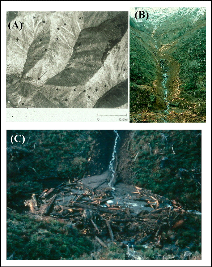Figure 1. Photographs of debris flows in the Pacific Northwest. (A) Post fire debris flows originating from steep and convergent areas (e.g., Figure 3-2) and traveling through headwater streams in western Oregon. (B) A debris flow in a logged area in northwest Washington. (C) Debris flow deposit within a larger, fish bearing stream, Oregon Coast Range.

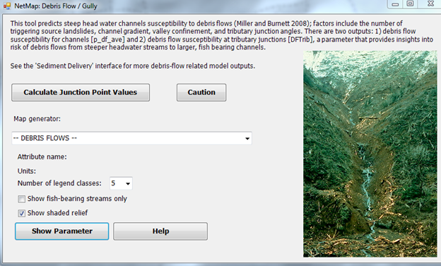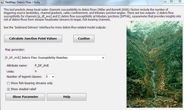Figure 2. NetMap's debris flow tool contains predictions for all stream reaches, but of greatest concern are headwater streams. Also included are debris flow probability in mainstem (fish bearing) channels from adjacent steeper tributaries (second attribute in dropdown list). The attribute "DF_Junct" or Debris Flow Susceptibility-Junctions can be used in NetMap Risk Analysis Tool to determine if and where debris flows overlap sensitive fish habitats. The delivery of debris flows to streams can be evalauted using NetMap's Delivery Tool. In addition, debris flow deposit survivability can be predicted and debris flow risk can be mapped onto junction points (by using "Calculate Junction Point Values", and see Figures 3 through 5 below for examples.

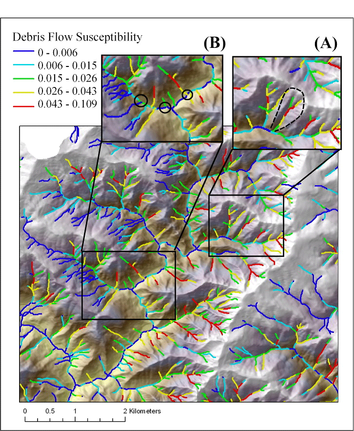Figure 3. Predicted debris flow susceptibilities are shown for a portion of the Wilson River basin. Downstream sequences of susceptibilities in headwater streams (A) can be used to differentiate one debris flow prone headwater stream from another (low-high might warrant more caution compared to high – low). The susceptibility of headwater streams immediately above a larger, fish bearing channel (B) can also be used to differentiate debris flow potential and possible impacts to larger channels. The downstream sequence of predicted susceptibilities can be used to estimate the likelihood of debris flows reaching a specified channel segment, such as fish habitat. For example, a headwater - upstream to downstream sequence debris flow susceptibility of low – high – low would be less of a concern compared to the sequence of low – moderate – high or moderate – high or simply overall high (A). In addition, one should focus on the predicted debris flow susceptibility of the segment located immediately upstream of the low- to high-order debris flow prone confluence. Headwater segments with high susceptibility immediately upstream of the confluence with a larger fish-bearing stream is of more concern compared to headwater segments with a lower susceptibility ( B).

Debris Flow Impacts to Fish Bearing Streams

To consider the effects of debris flows on channel morphology or in fish bearing streams, a user should focus on the predicted debris flow susceptibility of the segment located immediately upstream of the headwater-mainstem tributary confluence (in the headwater debris flow prone channel). Headwater segments with high susceptibility immediately upstream of the confluence with a larger fish-bearing stream is of more concern compared to headwater segments with a lower susceptibility.

NetMap contains a parameter to facilitate the analysis of patterns (juxtapositions) of headwater confluences prone to debris flows with fish bearing streams. The parameter Debris Flow Susceptibility - Junctions can be used to quickly identify confluences and hence associated fish habitat reaches at potential risk (Figures 4 and 5). The debris flow susceptibility-junction is a field that is mapped in the network (outside of headwater first- and second-order streams) that records the debris flow susceptibility value in the lowest part of the confluencing headwater channel. Debris flow susceptibility-junctions are mapped as a reach parameter (so that it can be used in several of NetMap’s tools, including Habitat Diversity and Channel Disturbance. Thus, the point of interest is the area at and in the immediate vicinity of the confluence of the headwater channel with the mainstem stream. In mainstem reaches that have more than one confluencing debris flow-prone headwater channel, the highest debris flow susceptibility value (from the lower most reach of the headwater channel) is reported in the reach file.

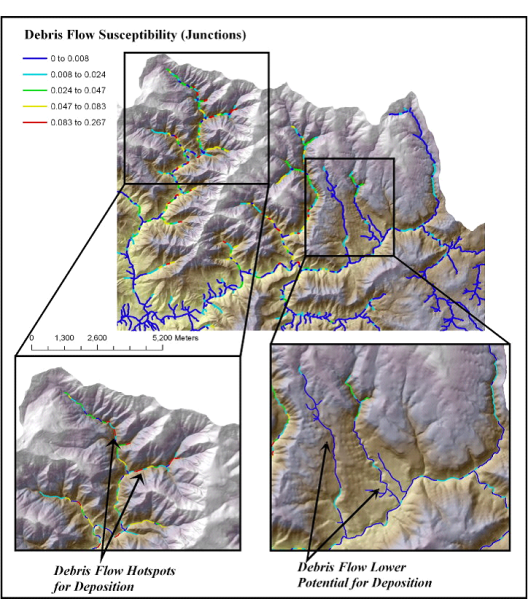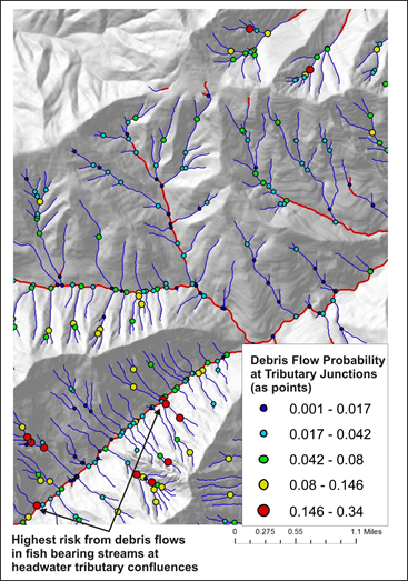Figure 4. “Debris flow susceptibility-junctions” is predicted for tributary confluences in a portion of the Wilson River basin (Oregon Coast Range). This type of prediction will facilitate comparison of debris flow susceptibility with other channel and habitat parameters (see Overlap Risk Tool).

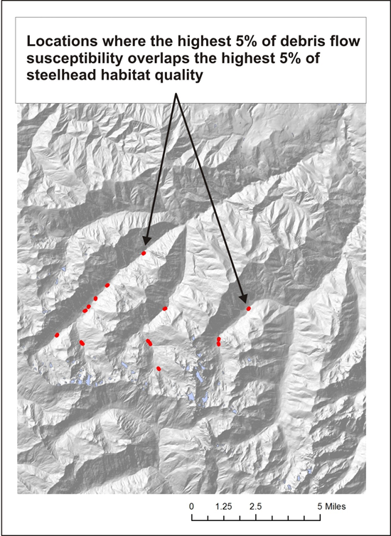Figure 5. An example of how the attribute "DF_Junct" or Debris Flow Susceptibility-Junctions can be used in NetMap Risk Analysis Tool to determine if and where debris flows overlap sensitive fish habitats. Shown are locations in a watershed in coastal Washington where the highest 5% of debris flow risk overlap the highest 5% of steelhead habitat quality.

Model Description (2/4): Debris Flow Risk in Streams using a Channel Gradient Threshold

Field Name: trav_ID; Common Name: Debris flow traversal (the probability of debris flows traversing channel grid cells)

Another model output is the the probability of debris flow traversal in individual channel cells, and it is based on a specified gradient threshold for that traversal (the default is 200% or all streams); use the Delivery tool to import this layer as well as specifying a new gradient threshold, such as for anadromous fish bearing streams, e.g., less than 10% for example. The amount of traversal with a delivery of 0.2 will be much higher compared to a channel delivery gradient threshold of 0.02. This refers to the length of debris flow track (and probability) than can reach into 2% streams and less; there are many more debris flows that can deliver to channels less than or equal to 20%.

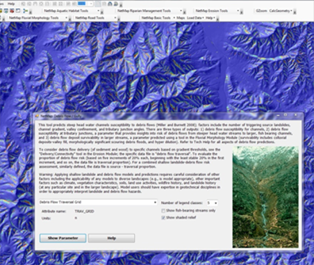Figure 6. Debris flow delivery (of sediment and wood) can be predicted to specified channel gradient thresholds, here shown for all channels (e.g., 200% channel gradient threshold).

Model Description (3/4): Proportion of Debris Flow Risk (watershed scale)

Field Name: travprop_ID.flt; Common Name: Traversal proportion grid

This tool allows a user to calculate the proportion of debris flow risk, in terms of traversal of stream segments, based on the cumulative distribution of values, starting at the maximum risk of traversal, e.g., the top 20%, the next highest 20% and so on (Figure 7). This parameter is sensitive to a user defined channel gradient threshold that defines "delivery" of sediment and wood to streams. Refer to the Delivery Tool for additional information. The default setting supplied with NetMap datasets is delivery to streams less than or equal to 200% (e.g., all streams).

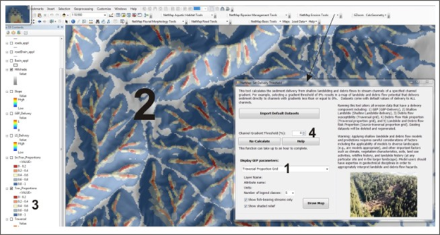Figure 7. Analyst can select the "traversal proportion grid" (1) to examine the proportion of debris flow runout risk in increments of 20% of the full distribution, such as the highest 20%, the next highest 20% and so on (2, 3). A user can specify a different channel gradient threshold to examine debris flow runout risk, e.g., runout to channels less than 8% (anadromous fish habitat), less than 20% (resident and anadromous fish habitat) etc.

Model Description (4/4): Proportion of Combined Shallow Landslide and Debris Flow Risk (watershed scale)

Field Name: proportions_ID; Common Name: Source Traversal proportion grid

Debris flow risk can also be combined with the risk of shallow failures, since shallow failures trigger debris flows in NetMap's models (Miller and Burnett 2007, 2008, Benda and Dunne 1997a). In this model, the proportion of risk from shallow landslides (see Shallow Failure parameter) is combined with the proportion of debris flow risk (see above Model 3/4). The resulting parameter predicts a combined risk factor for both (Figure 8). This parameter is sensitive to a user defined channel gradient threshold that defines "delivery" of sediment and wood to streams. Refer to the Delivery Tool for additional information. The default setting supplied with NetMap datasets is delivery to streams less than or equal to 200% (e.g., all streams).

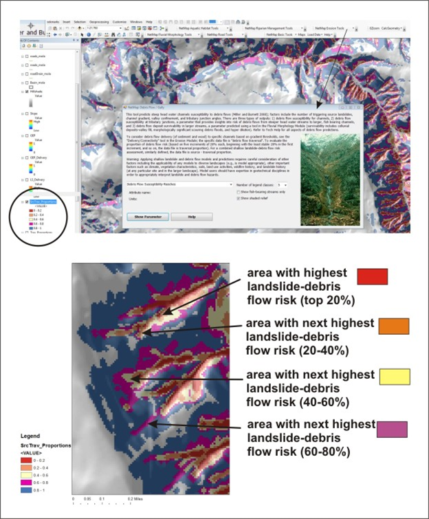Figure 8. NetMap's combined shallow landslide-debris flow risk index predicts areas in the landscape with different proportions of risk, starting with the most unstable and most likely to have debris flows (in increments of 20%, although that legend breakdown can be adjusted in ArcMap's symbology editor). In the example above, the red colored areas have the highest 20% of risk combined in both shallow landslide area (unchanneled hillsides) and debris flows in headwater streams. The orange areas contain the next highest 20% or risk. The red and orange areas combined contain 40% of the risk. To identify areas that contain 80% of the predicted combined landslide and debris flow risk, red, orange, yellow and purple areas would added together. This type of prediction is useful when considering managing landslide risk or when considering upslope source of large wood to streams (see Upslope Sources of Wood in the Riparian Management Tool).

Background

Debris-flow susceptibility values indicate the relative potential for debris flow movement through a reach. The susceptibility is relative because it is based solely on the specified mean landslide density (see Shallow Landslide), the topographic weighting term, and the probability for delivery from each hillslope pixel – there is no temporal component from which to directly calculate actual probabilities (e.g., recurrence intervals). The implications of a given debris-flow susceptibility vary with position in a channel network and with the gradient, size, and valley morphology of the receiving channel. For steep, headwater channels, a high debris-flow susceptibility implies a potential for debris flow scour. For lower gradient headwater channels and at tributary junctions, a high susceptibility implies a potential for debris-flow deposition. For mainstem channels, the consequences of debris-flow delivery vary with the potential for fluvial transport of the deposited material (Benda, 1990). The deposits may be long-lived in small, low-gradient channels, resulting in formation of debris fans. As channel size and/or gradient increase, the potential for erosion of debris-flow deposits increases. Boulder lags, truncated fans, and downstream fluvial deposition of debris-flow supplied material may be the only evidence of past debris flows. NetMap includes a function for predicting the fate (i.e., erosion) of debris flow deposits and a classification of potential debris flow effects in channels (see below).

NetMap’s debris flow model is empirically calibrated to Oregon Coast Range conditions (refer to Miller and Burnett 2007b). Debris flow runout is sensitive to forest cover with higher probabilities of debris flows associated with open (cleFieldut) cover compared to mature forests based on the empirical data used to calibrate the model. This is because mature forests are associated with fewer field observations of debris flow scour, more deposition, and shorter runout paths. This finding is consistent with previous studies of debris flow movement in the Oregon Coast Range (Ketcheson and Froelich 1978, May 2002). However, NetMap applies the debris flow runout model using mature forest canopy to produce a uniform prediction across entire landscapes (e.g., information on vegetation patterns and their change over time is not required).

Because of the empirical calibration, the debris flow model is most appropriate for coastal Oregon, although it could be applied to other humid mountain landscapes that are prone to debris flows in steep headwater streams. It is recommended that the probability ranking be changed to a “high likelihood” to a “low likelihood” of occurrence in other landscapes. Other factors need to be considered such as climate and vegetation.

A NetMap tool (e.g., Sort and Rank) allows for aggregating debris flow susceptibility at subbasin scales by creating cumulative distributions (CDFs) on the fly. The output then ranks subbasin by overall (average) debris flow risk (Figure 9).

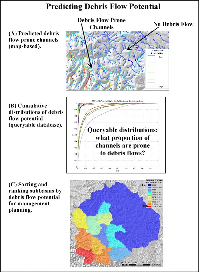Figure 9. The NetMap model for debris flows can be applied to specific landscapes. The model shown here was developed and empirically calibrated for the Oregon Coast Range but can be used in other landscapes as a relative ranking of debris flow runout risk. (A) Maps are produced indicating the locations of varying potential for debris flows at the individual hillslope scale. (B) Cumulative distribution functions (CDFs) of relative debris flow risk are created at the subbasin scale by another NetMap's Sort & Rank Tool. Such information can be used to sort and rank subbasins according to debris flow risk across landscapes (C). The model should have general applicability to other landscapes prone to debris flows.

NetMap contains a parameter to facilitate the analysis of patterns (juxtapositions) of headwater confluences prone to debris flows with fish bearing streams. The parameter Debris Flow Susceptibility - Junctions can be used to quickly identify confluences and hence associated fish habitat reaches at potential risk (Figure 4). The debris flow susceptibility-junction is a field that is mapped in the network (outside of headwater first- and second-order streams) that records the debris flow susceptibility value in the lowest part of the confluencing headwater channel. Debris flow susceptibility-junctions are mapped as a reach parameter (so that it can be used in several of NetMap’s tools, including Habitat Diversity and Channel Disturbance. Thus, the point of interest is the area at and in the immediate vicinity of the confluence of the headwater channel with the mainstem stream. In mainstem reaches that have more than one confluencing debris flow-prone headwater channel, the highest debris flow susceptibility value (from the lower most reach of the headwater channel) is reported in the reach file.

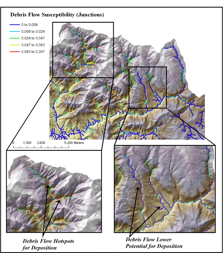Figure 10. “Debris flow susceptibility-junctions” is predicted for tributary confluences in a portion of the Wilson River basin (Oregon Coast Range). This type of prediction will facilitate comparison of debris flow susceptibility with other channel and habitat parameters.

Debris flow movement declines with decreasing channel slope (Swanson and Lienkaemper 1978, Benda and Cundy 1990, Fannin and Rollerson 1993, Fannin and Wise 2001), declines at sharp-angled tributary junctions (Benda and Cundy 1990), is less in large forests and longer in clearcuts (Ketcheson and Froelich 1978, May 2002), and increases with larger volumes (Benda and Cundy 1990). Similar to the empirically calibrated landslide model, predictions of debris flows in NetMap are based on four topographic attributes derived from field studies in the Oregon Coast Range (using data from Robison et al. 1999) and include 1) channel slope, 2) valley width or confinement, 3) angles of tributary junctions, and 4) cumulative length of scour and deposition (i.e., rate of volume increase or decrease) (refer to Miller et al. 2003, and Miller and Burnett 2007b). In the model, debris flow runout is separated into zones of scour, transitional flow, and deposition. The functional relationships between debris flow scour and deposition and the four topographic factors are based on field reseFieldh that has illustrated the physical constraints on debris flow travel.

There are a variety of models developed to predict debris flows and their movement and deposition in headwater streams primarily in humid landscapes (Benda and Cundy 1990, Hungr et al. 1984, Fannin and Rollerson 1993, Lancaster et al. 2001). Most of these models require information on network characteristics of headwater systems such as channel gradients and tributary junction angles.

The debris flow susceptibility model reveals a high degree of variability within individual headwater streams and across a watershed, such as the Wilson (Figure 4). Debris flow “probabilities”, or more accurately described as “susceptibilities” since it provides a relative index (and not precise probabilities), can be used in several different ways to support ODF management of landslide and debris flow prone areas.

Ecological Implications

Debris flows are a significant component of sediment budgets in many mountain landscapes (Dietrich and Dunne 1978; Swanson et al. 1982; Wohl and Pearthee 1991) and they can cause erosion to be highly episodic (Benda and Dunne 1997a; Kirchner et al. 2001). In certain landscapes, low-order channels prone to debris flows comprise up to 80% of a channel network, and hence network topology can influence the spatial diversity of channel and valley morphologies (Benda and Dunne 1997b). In depositional areas, debris flows construct levees (Canon and Bonny 1902); build fans at tributary junctions (Dietrich and Dunne 1978); create boulder deposits along fan margins (Benda 1990; Wohl and Pearthree 1991); form ponds at fan constrictions (Everest and Meehan 1981); create wide valley floors (Grant and Swanson 1995); force channel meanders (Benda 1990); and spates of debris flows can lead to widespread channel aggradation and formation of terraces (Wohl and Pearthee 1991; Robert and Church 1986; Miller and Benda 2000). In addition, debris flows can incorporate logs and whole trees that have accumulated in low-order channels over decades to centuries and they deposit them on fans, valley floors, and in channels at low-order confluences (Swanson and Lienkaemper 1978; Hogan et al. 1998; May 1998).

Road construction and timber harvest have increased the occurrence of debris flows in some landscapes by lowering hillslope stability (Burroughs and Thomas 1977). In some cases, debris flows have increased their travel distances due to the absence of large trees along flow paths (Ketcheson and Froelich 1978; May 1998). Increased occurrence of debris flows due to timber harvest and logging roads has raised concerns about impacts to fishes and other aquatic life. Negative effects of debris flows may include immediate burial of existing habitat and direct mortality of aquatic biota; increased fine sediment in gravels onsite and downstream that suffocates fish eggs in gravel (Everest et al. 1987; Scrivener and Brownlee 1989); increased bedload transport and lateral channel movement due to heightened sediment supply that scours fish eggs; and loss of pools that reduces rearing habitat (Frissel and Nawa, 1992; Hogan et al. 1998).

Debris flows are also a “disturbance” when viewed by ecologists (Swanson et al. 1988) and the pivotal role of certain types of disturbances in maintaining productivity and diversity in aquatic ecosystems is gaining increasing recognition (Resh et al. 1988, Reeves et al. 1995). Beneficial effects of debris flows on aquatic systems include formation of ponds that become occupied by fish and beaver (Everest and Meehan 1981); release of nutrients due to buried organics in anaerobic environments (Sedell and Dahm 1984); deposition of woody debris that creates sediment wedges and forms pools (Hogan et al. 1998); deposition of boulders that trap sediments and create complex habitats (Reeves et al. 1995); formation of wider valley floors that contain larger floodplains (Grant and Swanson 1995); and increased biological productivity (Roghair et al. 2002). Spates of debris flows may also contribute to watershed-scale habitat diversity, including in riparian forests (Nierenberg and Hibbs 2000; Nakamura and Swanson 2002).

To gain a longer-term perspective on episodic erosion in humid mountain landscapes, the occurrence of debris flows and sediment routing at the scale of a sixth- order network over centuries was investigated using computer models (Benda and Dunne 1997; U. S. F. S 2002). The models predict that large volumes of sediment are concentrated in parts of the channel network, particularly near tributary junctions (i.e., low-order to high-order confluences), during infrequent periods of intense hillslope erosion following forest fires and large storms. The concentration of sediment at low-order confluences was referred to as ‘stationary sediment waves’ to extend the definition of fans to include their temporally variable influences on channel morphology and to distinguish them from waves of sediment that migrate through a network. A later theoretical analysis of the long-term mass balance of in-stream wood indicated the potential importance of debris flows as a wood recruitment agent in larger channels (Benda and Sias in press), a prediction that was preceded and motivated by field studies indicating the same conclusion (Swanson and Lienkaemper 1978; Hogan et al. 1998).

Despite the history of field work and modeling, the effects of debris flows on channel and valley morphology, particularly as it pertains to riverine ecology, remain an outstanding question. For example, none of the existing models for predicting the occurrence of shallow landslides (Montgomery and Dietrich 1994) and transport distance of debris flows (Benda and Cundy 1990, Fannin and Wise 2001) consider or predict the morphological or ecological consequences in rivers. This reduces the ability of geomorphology to effectively participate in interdisciplinary collaborations that are aimed at understanding natural environments and human alterations of them. In addition, although the potential for tributary confluences to play a key role in riverine ecology has been acknowledged, little supportive empirical information exists (Fisher 1997).

Made with help of Dr.Explain