| < Previous page | Next page > |
ChannelGeneric Erosion Potential (GEP) - Channel (Fish-Eye View
Parameter Description: The Generic Erosion Potential is displayed at the scale of individual channel segments, offering a "fish-eye" view of erosion potential, at the scale of drainage wings adjacent to the channel.
GEP is the susceptibility of hillslopes to shallow failure and to gullying based on a topographic index combining slope steepness with slope convergence (GEP). Slope steepness is a fundamental control on erosion potential. Convergence causes surface and subsurface flow to become concentrated and therefore contributes to erosion potential (See Generic Erosion Potential (GEP)-Hillslope for more details).
Channel based erosion potential allows analysts to quickly identify individual hillsides (and adjacent channels that are the recipient of the erosion products [inorganic and organic material]) that have the highest erosion potential (for example, the top 5% of a watershed's erosion potential); see Habitat-Stressor Overlap tool. An analyst can then quickly identify overlaps between the top 5% of erosion potential and the top 5% of fish habitat quality, resulting in a risk assessment, that can be used in the context of resource user management. See Figures 4 and 5 below.
There are four model components: (1) GEP without sediment delivery to streams considered at the scale of individual channel segments (scaled by area, GEP/km2), (2) GEP without sediment delivery to streams routed or aggregated downstream, revealing erosion potential patterns at any basin scale defined by the stream network (i.e., bottom of first-order basin, bottom of second-order basin, etc., and at any place in between); and 3 & 4) GEP with sediment delivery to streams considered at the scale of individual stream segments and routed downstream. Note that in the context of sediment delivery, a user may define the channel gradient threshold that governs delivery, e.g., a delivery threshold of less than or equal to 20% will reveal more areas that can deliver compared to a delivery threshold of 10% (see Delivery Tool).
Important Notice: This erosion model is not calibrated to any particular area. Although the model employs universal topographic indicators of shallow landslide potential (and also gully potential), increased accuracy and resolution can be obtained when the GEP index is calibrated using local data (georeferenced locations of landslides or gullies). A landslide calibration tool is planned for NetMap in later 2014. Also see Warning about using Slope Stability Models.
Data Type: Line
Field Name: GEP; Common Name: GEP per channel reach
Field Name: GEP_CUM; Common Name: GEP aggregated (or routed) downstream
Field Name: GEPDEL; Common Name: GEP delivered per channel reach
Field Name: GEPDEL_CUM; Common Name: GEP delivered aggregated downstream
Units: Numerical values, range from 0 to >1, but scaled by area, in GEP units/km2
NetMap Module/Tool: Erosion Module/Generic Erosion Potential
Model Description: Values for Generic Erosion Potential (GEP) (hillslope grid) are summarized within individual ‘Drainage Wings’ on both sides of the channel and summarized as a reach attribute (GEP_segment). Segment GEP values are then aggregated downstream (GEP_aggregated) revealing a channel eye view of hillslope erosion potential (GEP) at any watershed scale defined by the stream network.
NetMap’s aggregation tool reports GEP to individual stream segments (GEP units/km2) and also routes that information downstream. In NetMap, each channel segment’s local contributing drainage area is defined on both sides of the channel (called drainage wings, Figure 1) and information contained on those hillsides is reported to the channel segment (Figure 2). That information is then routed downstream.
GEP values are weighed by drainage area as in GEP/km2. Stream segment scale and aggregated downstream values of erosion potential can be used in other NetMap tools, for example when searching for overlaps between high erosion potential and quality fish habitats. Tool use is described in Figure 3.
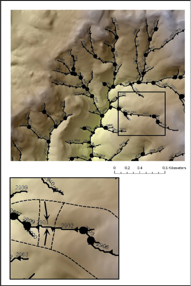 Figure 1. NetMap applies a universal data structure to all of its watershed analyses. This involves organizing river networks into stream segments (with Ids), confluence nodes, and local contributing drainage areas. Hillslope and channel information is routing downstream revealing patterns across multiple scales.
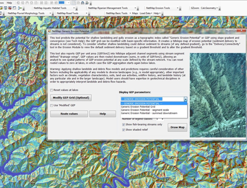 Figure 2. In NetMap, certain hillslope parameters are aggregated into the nearest and downslope stream channel segment (1) so that they can be used with other NetMap tools. NetMap determines the contributing hillslope area that drains into channel segments (on both sides of channels) that range in length from 20 to 200 m (2). The algorithm then determines the amount of road length that intersects those contributing areas and calculates a channel segment-based road density (km km-2) (3). NetMap also calculates similar densities for erosion potential (GEP), shallow landslide potential, and fire risk (or burn severity). NetMap also aggregates segment-based values downstream throughout a river network, yielding drainage area weighted values for road density, erosion density, landslide potential density, forest age, and fire risk (or burn severity) density. This is used in the Search for Overlaps tool. For example, an analyst can search for the highest 10% of erosion potential and where it overlaps with the highest 10% of fish habitat quality. Or where the top 5% of erosion potential overlaps with the top 5% of road density.
Use of the Tool
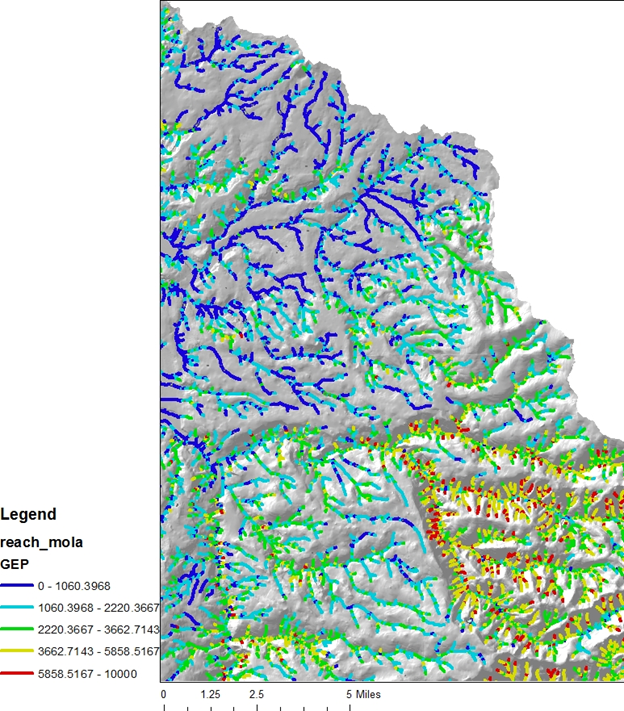 Figure 3. Once the Generic Erosion Potential data have been imported, five types of attributes are available for display: (1) the hillside prediction without the sediment delivery component (Grid), (2) the in-stream value without sediment delivery (accumulated from both sides of the channel, via Drainage Wings), (3) the downstream routed or aggregated values without sediment delivery, and (4, 5 and 6) the hillside (grid) and two channel values of GEP with delivery. Reach scale GEP values can be routed (after the first time when it was done automatically) and values can be reset at lakes if required (the default data when first loaded in a dataset is no reset at lakes) see Routing Tool. A modified GEP prediction can be made if a user supplies a set of polygons that have multipliers of GEP values (increases or decreases), and this attribute can be routed downstream or upstream; GEP based sediment yield predictions (t/km2/yr) can also be predicted using the modification procedure. To change the channel gradient threshold value to calculate sediment delivery, see Delivery Tool.
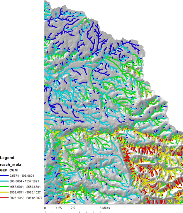 Figure 4. This example shows GEP values reported to individual stream segments, offering a stream- or fish-eye view of erosion potential from adjacent hillsides (using Drainage Wings). A large difference in hillside erosion potential is apparent in a N-S transect. Consequently, stream morphology, including tributary junctions, should have significantly different morphologies.
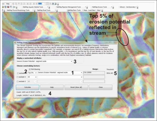 Figure 5. This example shows GEP values reported to individual stream segments and routed or aggregated downstream, offering a stream- or fish-eye view of erosion potential from upbasin areas, A large difference in hillside erosion potential is apparent in a N-S transect.
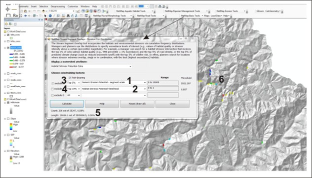 Figure 6. Use NetMap's Stressor Overlap Tool to quickly identify locations of the highest erosion potential. An analyst selects from the statistical distribution of erosion potential (1) from the drop down list (2), in this example the top 5%. The count of channel segments and their total length is shown (4). The threshold erosion (GEP) value is displayed (5). This analysis can be extended to stressor - habitat relationships, i.e., where does the highest erosion potential overlap the highest quality or most sensitive fish habitats (see Figure 6).
 Figure 6. In this example, a user selects the channel Generic Erosion Potential (GEP) value (1) and steelhead habitat (2), created using the habitat tool. They then select the highest 5% of erosion potential (3) and the highest 10% of fish habitat quality (4). The corresponding overlaps identify 206 stream segments or about 0.6% of the total channel length (5). Results are displayed in the map (6). Such habitat-stressor analyses can be used to identify high risk areas in the context of resource use management.
|