| < Previous page | Next page > |
Road Erosion/Sediment Delivery (READI)Road Erosion and Sediment Delivery Index (READI)
Parameter Description: The ability of roads to generate runoff, surface erosion and sediment delivery to streams is predicted by NetMap's READI model. At the scale of individual road segments, READI can be used as a dimensionless index on inherent erosion potential to prioritize road segments for field validation, maintenance and remediation, but calibration to field measured erosion rates can increase accuracy and be used to predict sediment yields (e.g., kg/storm or t/storm or dimensionless units/storm; the time unit is "storm" since READI is run on a per storm basis, typically a "design storm". READI can also be calibrated using field measured sediment transport distances or sediment plume lengths. READI can be run over mutlipe storms, manually, to calculate a per annum sediment yield.
Additionally, READI includes an optimization component that is used to predict where additional road drains can be strategically placed to further disconnect road segments from streams and where road maintenance and upgrades can reduce sediment delivery. When using READI to predict location of new drains, one MUST consider the potential for the new drain runoff to trigger gullies, landslides and debris flows. See below for a description of READI in the context of slope stability.
READI can be used in post fire environments, using decreased soil infiltration, to identify roads that can have increased road-stream connectivity post fire, thus informing post fire mitigation. READI can also be used to help understand how climate change can exacerbate road impacts in watersheds by using an altered climate.
Data Type: Road layer, Stream layer
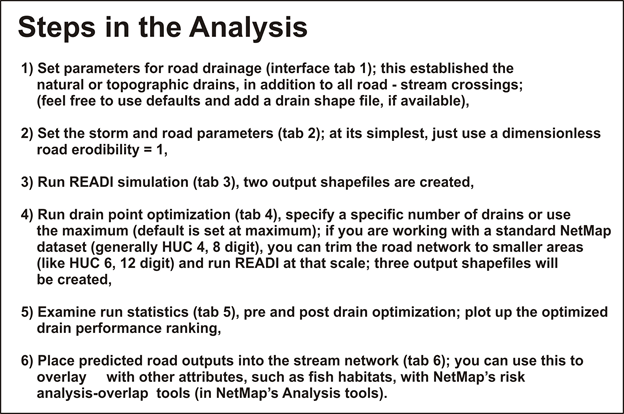
Begin Analysis:
READI_ID = road line layer, will have added drain points; a road layer broken up into hydrologically discreet segments based on road-stream intersections and high and low points along the topography (referred to as natural drains, and see here); (ID refers to NetMap's vritual watershed dataset name)
READIout_DrainPoints_ID = drain point shapefile, can have added drain points (a road layer broken up into hydrologically discreet segments based on road-stream intersections and high and low points along the topography [referred to as natural drains, and see here]); this layer is not loaded using the tool, but exists in the NetMap dataset folder Run READI Simulation:
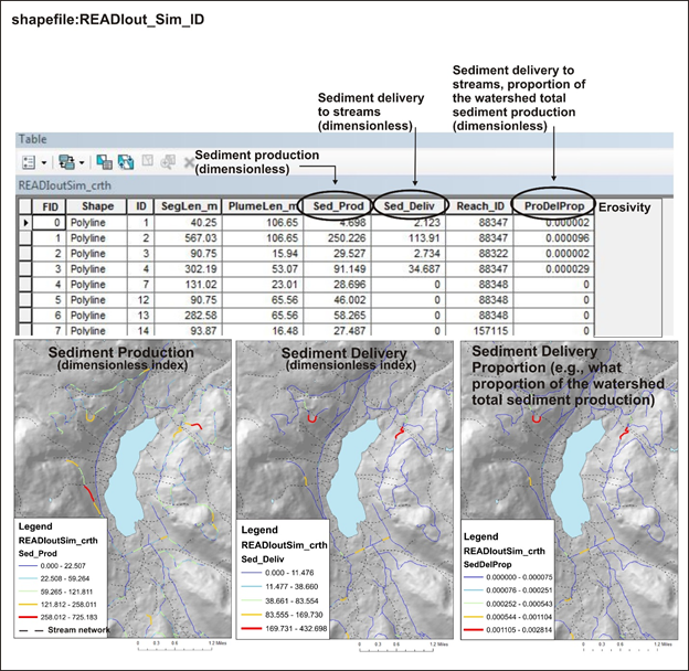
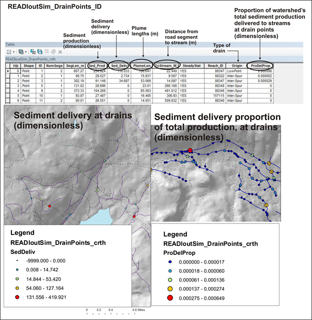
READIoutSim_ID = road layer (READI_ID) with output attributes including sediment production and sediment delivery to streams (see output ArcMap attribute tables below) READIoutSim_DrainPoints_ID = output drain points with attributes including sediment production and sediment delivery to streams (see output ArcMap attribute tables below) Generate Optimized Drain Locations and Optimized Locations for Road Surface Remediation:
READIout_DrainsToAdd_ID = Select those you want to use to rerun the simulation, they are sorted in the attribute table by effectiveness (at reducing road sediment delivery); Run READI simulation with Optimized Drain Points:
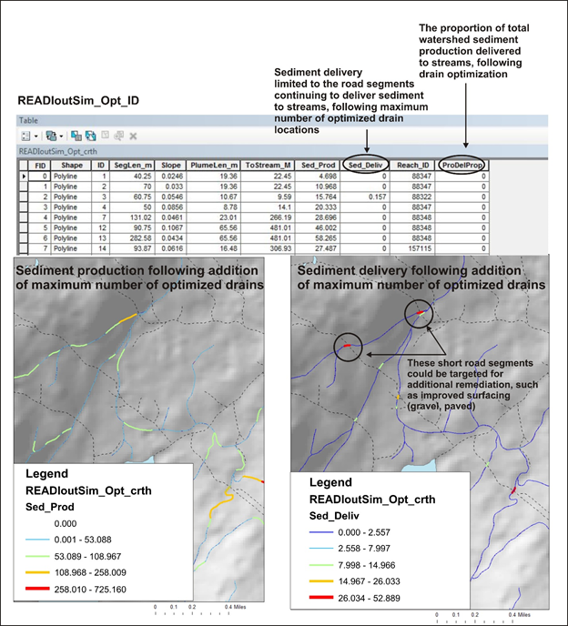
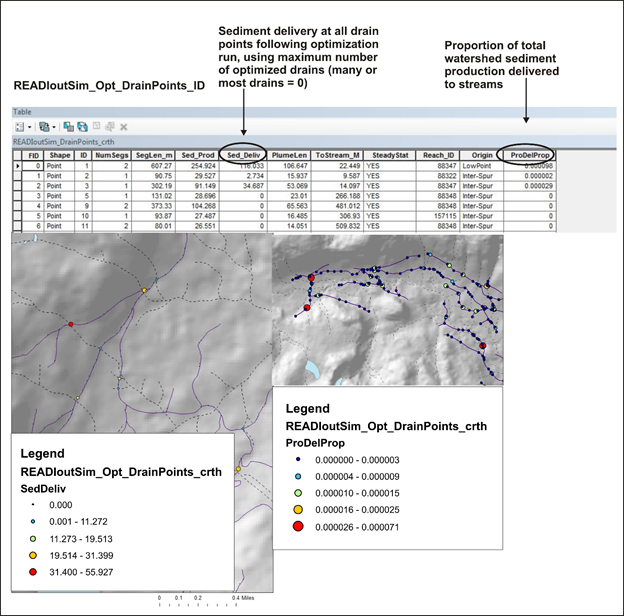
READIoutSim_OPT_ID = model output with attributes including sediment production and sediment delivery to streams (see output ArcMap attribute tables below) READIoutim_OPT_DrainPoints_ID = model output with attributes including sediment production and sediment delivery to streams (see output ArcMap attribute tables below) Units: Variable: READI can be applied as a dimensionless index (by setting E = 1) or given calibration in units of kg/yr or tons/yr etc.
NetMap Module/Tool: Erosion Processes/Road Surface Erosion
Model Description:
See draft paper here.
The road network (lines) is first broken at pixel cell boundaries. The individual, approximately pixel scale road cells, are then re-aggregated into hydrologically connected segments (tens to a hundreds of meters in length) that represent water flow paths from high (topographic) points to low (pour) points or to defined streams (see here). These hydrological road segments can be viewed in terms of their drainage diversion potential. For example, in the absence of secondary road drainage structures, the drainage diversion road segments should indicate the water diversion potential of any road segment, particularly under conditions such as during large storms or following wildfires. Refer to NetMap’s Road Drainage Diversion Potential parameter.
f
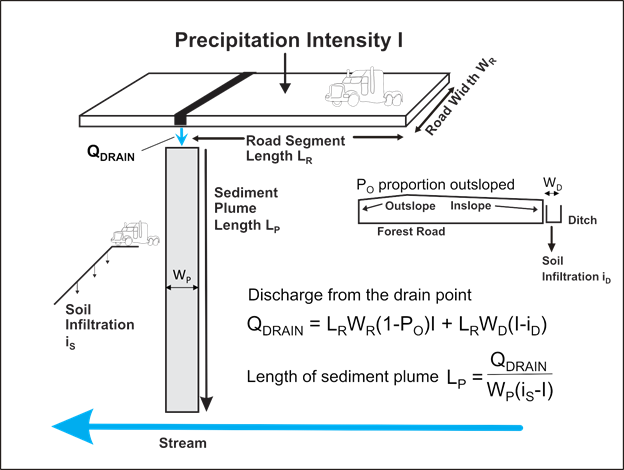 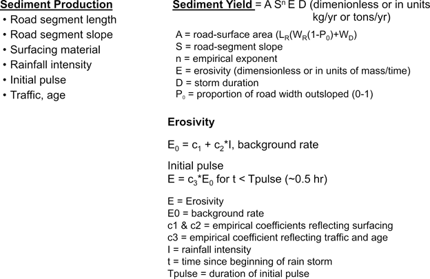 Figure 2. READI predicts road water runoff by multiplying road segment length by road width and rainfall intensity (m/yr) in units of m3/hr; the runoff can be adjusted by the proportion of road width outsloped. A water/sediment plume is
predicted that has a default rectangular shape (other shapes could be used) with an assigned plume width. Soil infiltration occurs along the plume; the model requires that rainfall intensity < soil infiltration capacity, otherwise there is Hortonian overland flow and unlimited sediment transport distances. Delivery of sediment and water to a stream is dependent on calculated plume length. Water delivery is based on integration of a hydrograph at the base of the plume. Sediment delivery is calculated by integrating sediment production from the road surface multiplied by a delivered proportion that is a function of the ratio of distance-to-stream and plume length; PD = c1*EXP(-c2*(LS/LP)) + c3 (LS is distance to stream). It is assumed that if LS/LP < 1.0, PD = 0, and that PD cannot exceed 1.0. Supporting literature: Croke et al., 2005; Ketcheson and Megahan, 1996. The predicted distribution of plume lengths can be calibrated using field measured plume lengths.
Erosivity is calculated as a base rate E0, and a “pulse” rate that may occur at the beginning of a storm, during which fine sediment accumulated since the last storm is flushed off the road surface. The base rate is calculated as E0 = c1 + c2*I, where I is rainfall intensity. The initial pulse is represented as a multiplicative increase of E0: Epulse = c3*E0, applied for a time Tpulse at the beginning of the storm. This model provides a simple representation of the behavior observed in numerous monitoring experiments, both for natural and artificial rainfall (e.g., van Meerveld et al., 2014). To set a constant background rate unaffected by rainfall intensity, set c2 to zero. To ignore the initial pulse, set c3 to zero.
Erosivity coefficients are also indicated for each road segment as data fields in the originating road shape file.
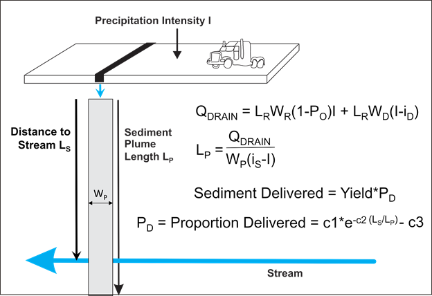 Figure 3. The proportion of sediment delivered to the stream is governed by a non linear relationship between predicted plume length and distance to stream.
READI Model Interface
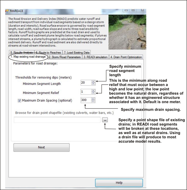
 INTERFACE TAB 1
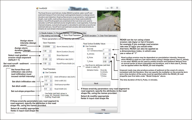
 TAB 2
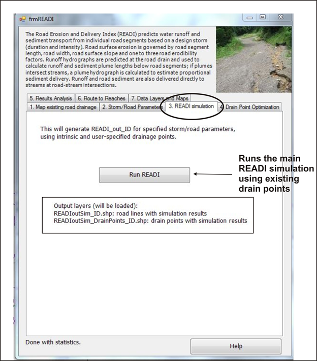
 TAB 3
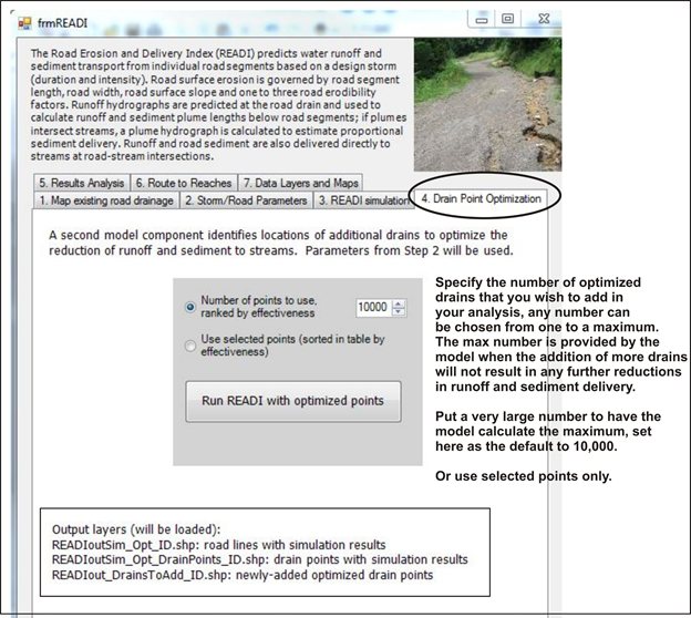
 TAB 4
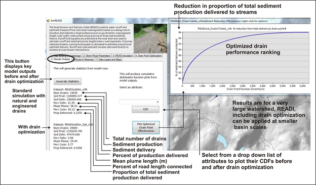
 TAB 5
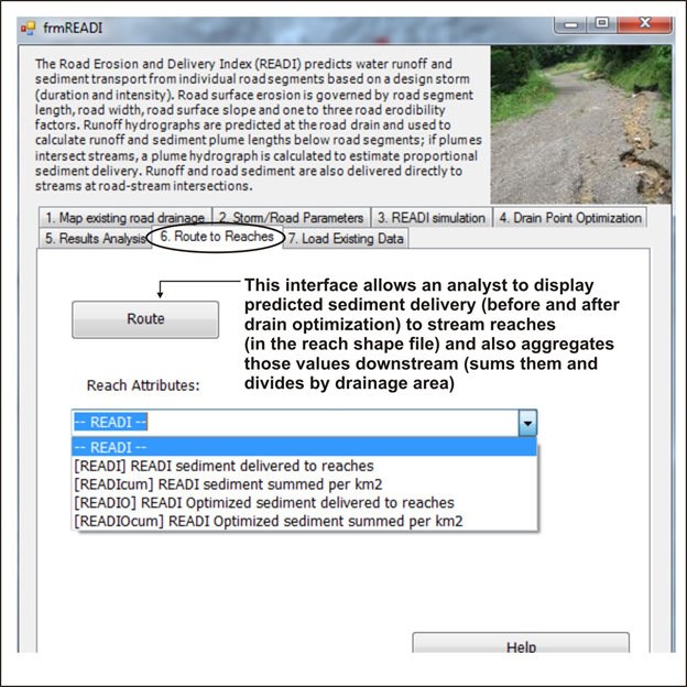
 TAB 6
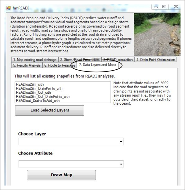
 TAB 7
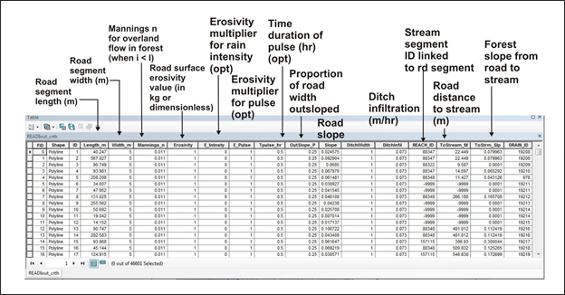
 Model Inputs Shapefile (READIout_ID); for reference purposes
 Key model output (for additional output parameters, refer to Appendix below).
Road Segments
 Road Drain Points
 When you run the READI Optimization Module (for strategically locating new drains to maximize sediment reduction effectiveness, here
are you key data (additional attributes in the shapefiles are shown in the Appendix, and end of page).
Road Segments
 Road Drain Points
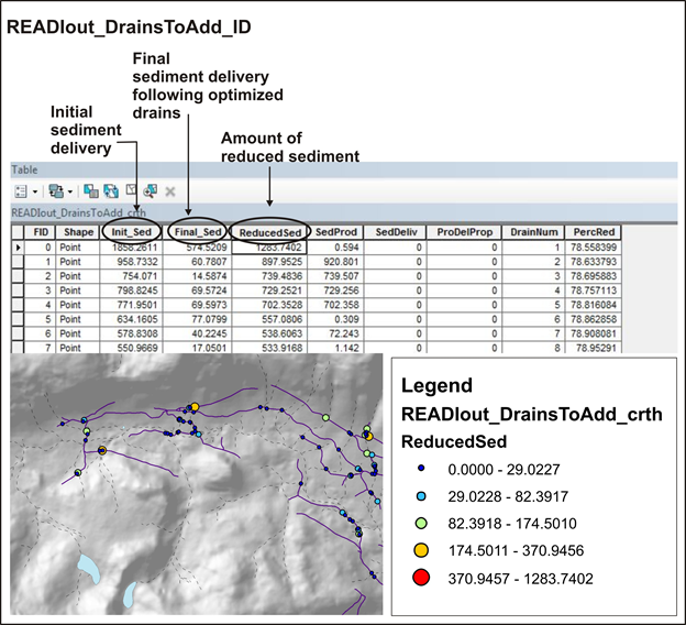
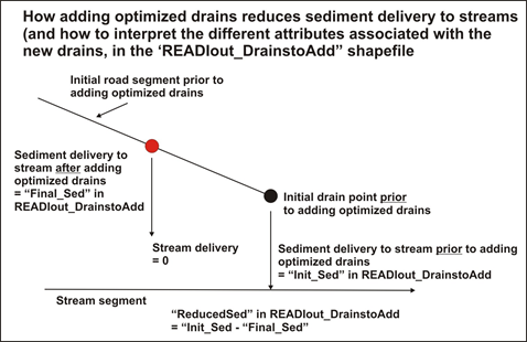
 Optimized Drains to Add (Points)
An analyst can use the attributes in the "drains to add" shapefile to prioritize placements of new drains to eliminate or reduce sediment delivery. See figures below.
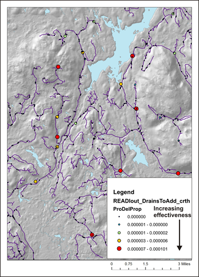
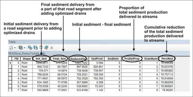   Another way is to use 'ProDelProp' and prioritize by the relative reduction in the proportion of total sediment production delivered to streams.
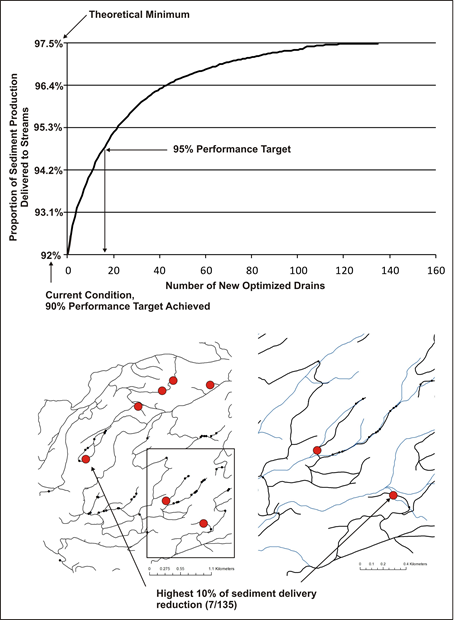
 New optimized drains are ranked according to effectiveness, the first ones in the queue are the most effective at eliminating or reducing sediment delivery, their effectiveness drops off with increasing number of drains, see example below.
 READI and Slope Stability
Using NetMap, placement of new drains must consider the potential for the new drain to trigger new gullies, landslides and debris flows. Two approaches are recommended. (1) The scientific literature identifies the use of the slope-area product, with area being the road surface segment area and the slope the hillslope gradient measured below the drain point (Montgomery 1994; Croke and Mockler 2001; Rakken et al. 2008). Thus, READI includes an attribute "slope area"; the higher the values the greater the potential that new drain runoff can trigger a gully or landslide. It is recommended that the attribute of reduced sediment of new drains by overlaid on top of the slope area attribute using a scheme shown in the figure below.
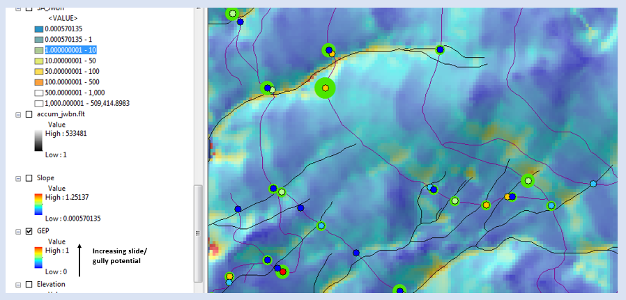
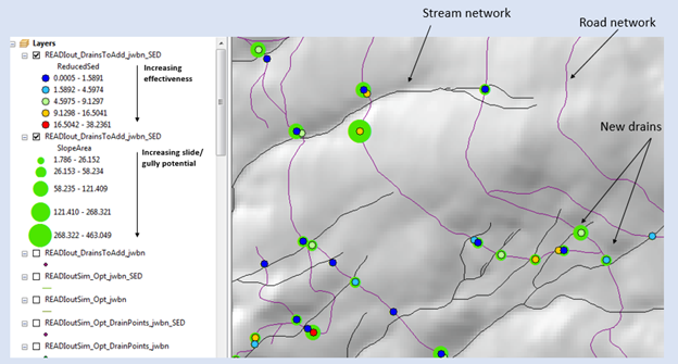 READI reduced sediment for new optimized drains overlaid onto predicted slope area product indicating the relative likelihood of new drain runoff to trigger gullies or landslides. When considering placement of new drains, NetMap Generic Erosion Potential attribute should also be used, in conjunction with READI new drain attributes and the slope area product. See figure below.
 Prioritizing Upgrades to Forest Road Surfacing
One can also prioritize where new road surfacing or other road surface erosion reduction strategies could be applied, and priortize them. For this exercise, it is best to create maps of predicted sediment delivery before or after calculating effects of adding new, optimized drains, and use those maps to identify those road segments with the highest predicted delivery. Then consider, based on the existing surfacing, whether upgrading surfacing, say from native to gravel, will reduce predicted sediment delivery. A map of prioritzation could be developed.
Model Application Example:
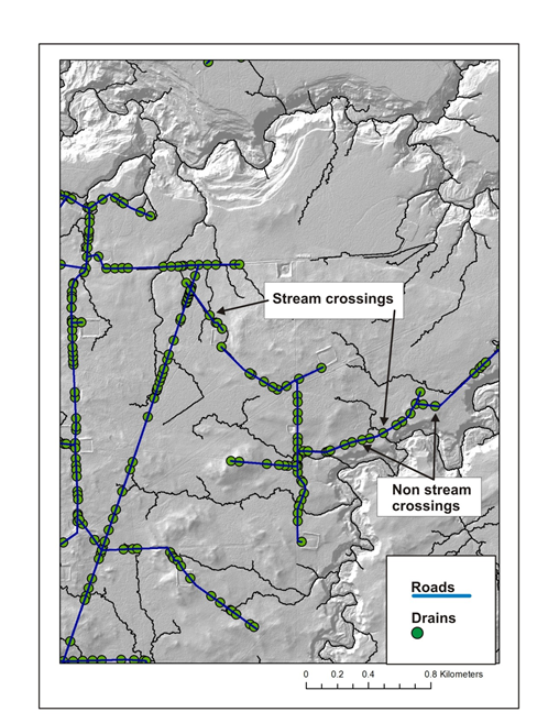 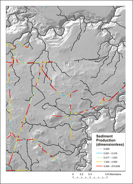 Figure. Starting drains either using the model, or loaded Figure. Predicted sediment production.
GPS drain points, referred to as natural or intrinsic drains. 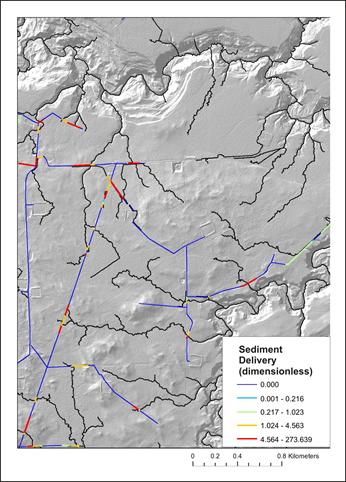 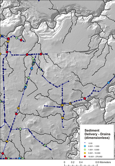 Figure. Predicted sediment delivery to streams (yo set to 1). Figure. Sediment delivery predicted at individual drain points.
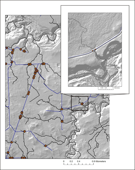 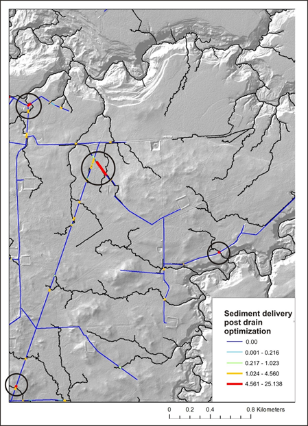 Figure. Optimized new road drain locations (added to natural Figure. Predicted sediment delivery following new drain optimization.
drains (see Figure above). 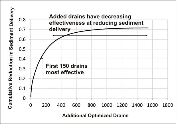 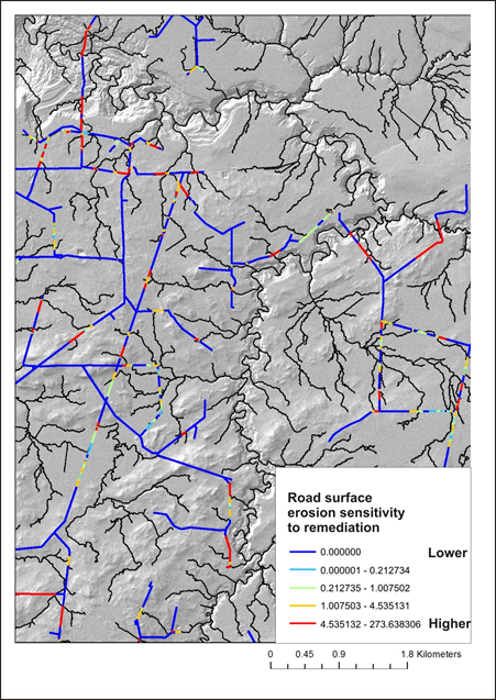 Figure. The cumulative effectiveness of adding new optimized Figure. Relative effectiveness of road surface improvements in reducing erosion.
drain points.
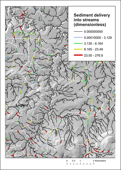 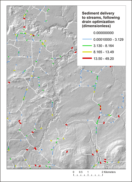 Figure. Predicted sediment delivery using non optimized drains Figure. Predicted sediment delivery using added optimized drains reported to reaches.
displayed in stream reaches (in NetMap's reach shapefile). Table. Example summary of READI outputs in the Simonette River watershed.
Model Technical Background (paper in prep, May 2016)
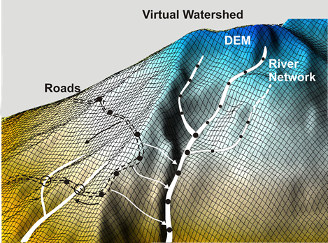 Figure 1. READI requires NetMap's virtual watershed data structure to be implemented. Road segments (GIS road layer) are first broken at pixel cell boundaries and then re-aggregated into hydrologically discreet segments based on
road-stream intersections (using NetMap's synthetic stream layer). Empirical studies find that water and sediment yields from forest roads are extremely variable, with sediment production highly sensitive to details of road construction and maintenance (Luce and Black, 2001), to interactions of road and hillslope hydrology (Wemple and Jones, 2003), and to the combined time series of rainfall events and traffic (van Meerveld et al., 2014). Detailed information on these factors is typically lacking, so that predictions of sediment yield are highly uncertain (Skaugset et al., 2011).
Despite the challenges posed in accurately measuring or predicting water and sediment runoff from roads, these processes remain primary suspects in the factors degrading water and aquatic habitat quality. Hence, regulatory agencies specify standards for road construction and maintenance, and increasingly require that road networks be hydrologically disconnected from stream channels (e.g., 2016 California Forest Practice Rules, Chapters 923, 943, and 963).
Forest-road networks are vast. In heavily managed basins, the cumulative length of forest roads often exceeds that of fish-bearing streams. Analysis tools to identify potential problem areas and to prioritize locations for road maintenance and improvement are sorely needed to aid in planning and to direct efforts to those locations and those modifications that will provide the most benefit at the least cost.
Our goal is to create a numerical template for road-network analyses that can be used to anticipate effects of roads on channel characteristics and associated aquatic habitat. For this, we seek a conceptual representation of how road networks interact with processes of water and sediment movement in the context of basin topography, geology, and climate. We seek a parsimonious representation, so that it can be applied in areas with limited data to gain insight about these interactions, but must still include the primary factors that drive water and sediment production and delivery from roads to channels, so that it can reproduce the types of behavior observed in actual, real-life systems.
Model Description
Empirical studies highlight the variability and uncertainty in measures of sediment production and delivery to streams from road networks, but they also identify a set of processes by which sediment production and delivery occur. Sediment production from roads is driven by road-segment hydrology (Surfleet et al., 2011), which can be grouped into two primary runoff-generating processes: 1) infiltration excess overland flow on road surfaces, and 2) interception of shallow-subsurface saturated flow by cut banks (Wemple and Jones, 2003). Surface water generated through these processes flows over road and cut-bank surfaces, and through ditches, collecting sediment from these surfaces as it goes, and potentially eroding rills and triggering cut-bank slumps. Sediment-bearing water is then discharged directly to streams at stream crossings, or onto the forest flow where it may continue flowing as overland flow, leaving a plume of sediment in its wake (Hairsine et al., 2002; Ketcheson and Megahan, 1996), or in certain conditions, it may incise gullies or trigger landslides and debris flows (Montgomery, 1994). For now, we focus specifically on infiltration excess overland flow and overland-flow plumes of water and sediment emanating from drain points, but recognize that these other processes must also be included for a complete characterization of road-channel interactions (Jones et al., 2000).
A variety of factors are observed to influence runoff and sediment yield from forest roads:
· Discharge rates of water and sediment are related to the surface area contributing runoff,
· sediment yield is related to the steepness of the road segment (Luce and Black, 1999),
· sediment yield varies with road surfacing material, road age, and road maintenance (Barrett et al., 2012; Luce and Black, 2001)
· sediment yield increases with increasing rainfall intensity (van Meerveld et al., 2014),
· log-truck traffic increases sediment production (Miller, 2014; van Meerveld et al., 2014),
· sediment concentrations in road runoff tend to be high at the beginning of a storm and to taper off over time (van Meerveld et al., 2014)
· the proportion of sediment delivered to streams decreases as the distance of the road from the stream increases (Croke et al., 2005; Ketcheson and Megahan, 1996).
These relationships are not found in all studies, which perhaps highlights the difficulty of measuring all the interacting variables, but because they are observed in some studies, we recognize the need for options to incorporate these relationships into a template for examining road and channel network interactions. Likewise, we recognize that because of the myriad interactions involved, accurate predictions of sediment yield may not be feasible. Hence, we temper our expectations and seek spatial patterns of water and sediment discharge to channels from forest roads in terms of relative amounts, rather than absolute quantities.
We also recognize that analysis tools must provide calculations of sensitivity to changes in the parameters that influence runoff, sediment production, and delivery to the channel system. This capability can show how uncertainty in input values influences predicted patterns of sediment production and delivery. It can also show where changes in road characteristics, such as surface material or drain spacing, might have the greatest effect on spatial patterns of sediment delivery to channels.
To fully characterize road-channel interactions, analysis tools must operate over entire watersheds. To fully characterize road-ecosystem interactions, analysis tools must operate over multiple watersheds. We focus here on watershed-scale interactions. To do so, we need spatially referenced information for road and channel locations that is linked to basin topography. For this, we rely on the concept of a virtual watershed (Barquin et al., 2015; Benda et al., 2016): a digital representation that explicitly links channel networks to the landscapes they drain. Using NetMap (Benda et al., 2007), a software platform that implements a virtual watershed within a GIS and provides facilities for linking different hydrologic and geomorphic models, we can drape a vector road network onto a digital elevation model (DEM, Figure 1) and parse roads into discrete hydrologic segments, extending from a high point to a low point along the topographic profile traversed by the road (Figure 2). Road segment length and gradient are calculated, and the flow-path to the nearest stream channel is characterized. This capability provides the foundation on which to build a template for road-network analyses.
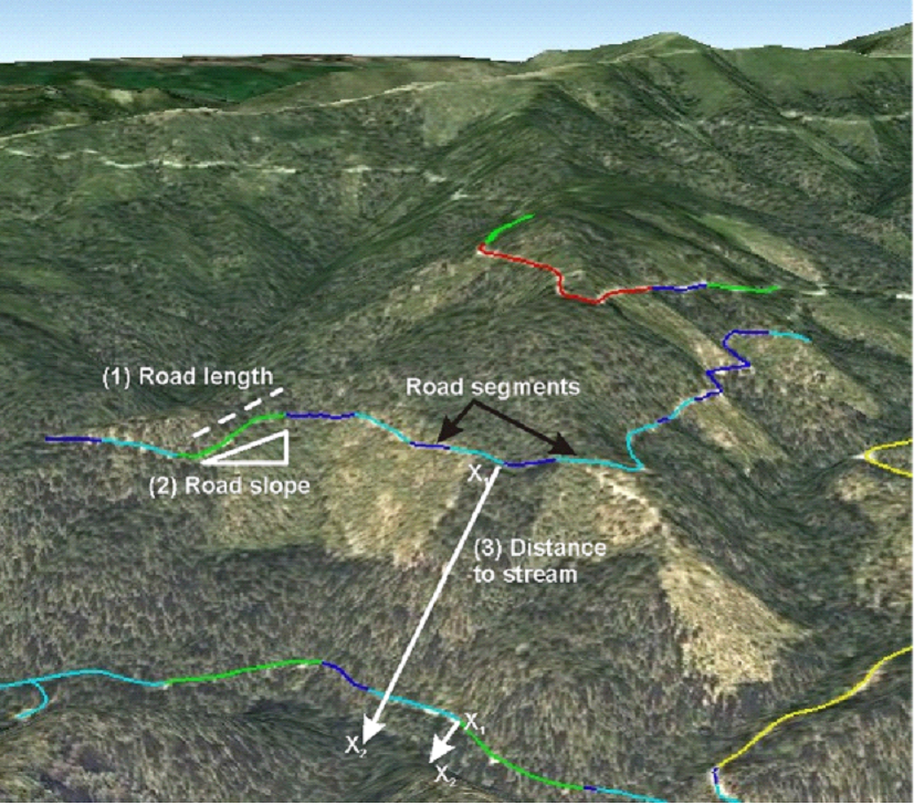 Figure 1. A vector road network can be draped onto a DEM. Road profiles can then be parsed into segments extending from high to low points. Low points are locations of drains that discharge sediment-bearing water either directly into streams or onto the forest floor. Additional constructed drain points, such as rolling dips or relief culverts, can also be placed on the road network. Road-segment length and slope, and the flow path to downslope streams, can be extracted from the DEM.
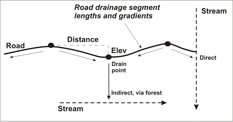 Figure 2. Road profiles obtained by draping a vector road network over a DEM are parsed into segments extending from high points, that act as local drainage divides for the road, to low points, that discharge sediment-bearing water that may be delivered directly to streams at road crossings or indirectly via flow paths through the forest floor.
To develop a prototype, we focus on a subset of the processes by which roads interact with streams: we examine runoff generated by infiltration excess overland flow and delivery via drain points that discharge water directly into stream channels or generate plumes of overland flow across the forest floor that may, or may not, flow to streams. We seek a representation of these processes that can be implemented using a minimum of input parameters, but with sufficient detail to reproduce the behavior generated by these processes (Figure 3). For this, we adopt the following simplifications:
· Rainfall events are characterized in terms of an average intensity I over storm duration D.
· Overland flow velocities are estimated using a kinematic wave approximation.
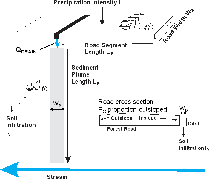 Figure 3. Representation of road-segment and sediment plume geometry.
Discharge
With these simplifications, discharge QR from a road-surface area providing flow to a drain is estimated as:
Here vR is average flow velocity over the road, t is time since beginning of rainfall, wR is width of the road prism, PO is the proportion of the road surface that is outsloped, so that wR(1-PO) gives the effective width of the road prism that contributes discharge to the drain point, LR is road-segment length, and I is rainfall intensity. We assume no infiltration into the road surface and make no accounting for depression storage, although such factors could be included in Equation .
Road geometry may specify a ditch of width wD and infiltration rate iD. Rainfall onto the ditch and infiltration into the base of the ditch add a discharge term:
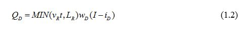 so that discharge from a road segment and its associated ditch is the sum:
With this simple model, discharge at the drain outlet increases linearly from initiation of the storm (t = 0) either until the time-to-concentration of the road segment (TCR = LR/vR), or for the duration of the storm D, whichever is shorter. If storm duration exceeds time-to-concentration (D > TCR), discharge remains constant from TCR until D. When the storm ceases at time t = D, discharge decreases linearly to zero at the rate vRwRIt over time interval TCR or D, whichever is smaller. We have applied the same average velocity for flow over the road surface and through the ditch. Channelized flow through a ditch is much faster than overland flow on the road surface, but generally the time-to-concentration for a road segment is considerably less than the storm duration, so that flow velocity has minor effect on total discharge.
NRCS Technical Release 55 (1986) provides an equation for estimating time-to-concentration (TC) for sheet flow derived using a kinematic wave approximation for flow velocity:
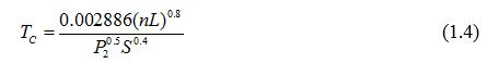 Here n is Manning’s roughness coefficient (Manning’s n), L is flow length (m), P is rainfall depth (m) for the 2-year recurrence interval, 24-hour storm, and S is surface slope. As an example, Table 3-1 in TR-55 specifies a Manning’s n of 0.011 for asphalt, gravel, and smooth bare-soil surfaces, and the intensity-duration curves for Mt. Shasta, CA (downloaded from the National Weather Service http://hdsc.nws.noaa.gov/hdsc/pfds/index.html), give the two-year, 24-hour storm depth as 0.105m, so a 100-m road segment with 5% slope has a time-to-concentration of approximately 0.03 hours and an average flow velocity v = L/TCR of about 3,333 m/hr, a leisurely walking pace. The time-to-concentration for a typical road segment is thus considerably less than the duration of a typical rainstorm, so that discharge at a drain point may be generally expressed as:
A single drain may receive flow from one or more road segments. If multiple road segments have flow to a drain, outflow from each segment is summed at the drain to produce the outflow hydrograph.
Discharge from the drain flows onto the forest floor and creates a plume of overland flow that extends downslope. Water from the plume infiltrates into the soil at a rate dictated by soil infiltration capacity and rainfall adds water to the plume from above at a rate given by rainfall intensity. Generally, the infiltration capacity of forest soils is considerably greater than even the most intense rainfall intensity, so the plume loses water with distance from the road and eventually disappears. Plume length LP is estimated as:
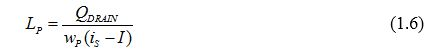 Here wP is average width of the plume and iS is soil infiltration capacity, so LPwPiS is the amount of water lost to infiltration along the plume and LPwPI is the amount of water added by rainfall per unit time.
From equation we find Qmin, the minimum discharge from the drain for the plume to extend length LS, the flow distance to a stream channel.
If discharge Qmin at the drain is reached at time t1, and the time to concentration for flow from the drain to the stream is TCS (using equation ), then discharge to the stream commences at time t1 + TCS with magnitude QDRAIN – Qmin. When the storm ceases at time t = D (the storm duration), rainfall input to the plume ceases and the minimum discharge from the drain required to maintain flow to the stream becomes:
Thus, once the storm stops, discharge to the stream persists only until discharge from the drain decreases to Qmin as specified by Equation .
Equations to provide the means to estimate discharge from a drain point to a stream channel as a function of storm intensity and duration and of road-segment geometry. At stream crossings, all the water discharged from a drain enters the stream. At other points, the proportion of water entering the stream depends on the geometry of the overland-flow plume, the distance to the stream, and the infiltration capacity of the soil. If distance to the stream is greater than the plume length, no overland flow is discharged to the stream.
Sediment Production
As listed at the beginning of this section, a variety of factors influence sediment production from roads, including road-surface area and slope, surfacing material, traffic levels, and rainfall intensity. To accommodate these factors, we specify sediment production from a road segment per unit time as:
Here A is road-segment surface area contributing sediment to a drain. Total sediment flux is calculated as the integral of PSED over time. Here
Here a and b are empirical constants; their magnitude reflects the erosivity of the road surface: larger values indicate more readily eroded material. For constant erosivity, b is set to zero. To represent an initial pulse of sediment, y0 is increased by a specified factor for a specified time TPulse:
The magnitude of coefficient c may be set to reflect processes that create an accumulation of erodible sediment over time, such as log-truck traffic. If c is set to one or TPulse to zero, there is no initial pulse.
Sediment Delivery
For road segments that drain to a stream crossing, all water and sediment enter the stream. For road segments with drain points onto the forest floor, discharge of water to the stream is assumed proportional to the ratio of potential plume length and the flow distance to the stream:
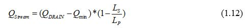 where Qmin is specified by Equation or , depending on time since beginning of the storm. The total volume of water discharged to the stream is then the integral of Equation over time.
For road segments that drain onto the forest floor, the quantity of material deposited in sediment plumes is found to increase in a nonlinear fashion with distance downslope. Ketcheson and Megahan (1996), for example, found that the ratio of volume deposited to total volume of the plume exhibited an exponential decrease with the downslope proportion of total plume length. In examining suspended sediment concentrations, Croke et al. (2005) also found an exponential decrease as a function of the proportion of total plume length. Hence, we estimate the discharge of sediment to the stream QSed as
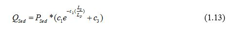 Here PSed is the sediment production rate specified in Equation , LS is flow distance to the stream, LP is the potential length of the plume specified in Equation , e is the base of the natural algorithm, and c1, c2, and c3 are empirically determined coefficients. Total sediment delivery is calculated as the integral of equation over time.
This conceptual model for generation of runoff by infiltration excess overland flow and delivery of water and sediment to streams via an overland-flow plume, implemented using Equations through , provides a means to estimate water and sediment delivery to a stream channel for a specified road segment for a storm of specified intensity and duration. This model includes only a subset of the processes recognized to generate sediment production and delivery – it lacks interception of subsurface flow by cut banks, or delivery via gullying or landsliding, for example – so it may not include the primary mechanisms in some landscapes. It is, however, the first step in building a comprehensive tool for road network analysis. It can be implemented within a virtual-landscape framework, and applied over all segments contained in a road network to show spatial patterns of connectivity to the stream-channel system. Primary parameters required for this model – road segment length, road segment slope, and flow distance from drain points to stream channels – are obtained by draping a road network over a DEM. Other road attributes (road-prism width, proportion outsloped, ditch width) can be obtained from records of road type, or from surveys of the road network, or set constant to represent average conditions. Parameters for sediment yield can be adjusted to account for differences in road surfacing and traffic levels. The model can be applied over a range of design storms to show how road-stream connectivity might change with storm characteristics.
Importantly, this framework can provide insight. If parameter values for sediment yield or road geometry are not well characterized, constant values can be applied and sensitivity of model results to changes in these values used to gage the need for more data collection. As we describe below, this framework can identify locations where construction of additional drains, or where application of gravel surfacing can be optimally applied to reduce connectivity to streams. It can show how reductions of soil infiltration rates due to wildfire might affect connectivity.
Barquin, J., Benda, L. E., Villan, F., Brown, L. E., Bonada, N., Vietes, D. R., Battin, T. J., Olden, J. D., Hughes, S. J., Gray, C., and Woodward, G., 2015, Coupling virtual watersheds with ecosystem services assessment: a 21st century platform to support river research and management: WIREs Water.
Barrett, B., Kosaka, R., and Tomberlin, D., 2012, Road surface erosion on the Jackson Demonstration State Forest: results of a pilot study, in Standiford, R. B., Weller, T. J., Piirto, D. D., and Stuart, J. D., eds., Proceedings of coast redwood forests in a changing California: A symposium for scientists and managers, Pacific Southwest Research Station, Forest Service, U.S. Department of Agriculture.
Benda, L., Miller, D., Barquin, J., McCleary, R. J., Cai, T., and Ji, Y., 2016, Building virtual watersheds: a global opportunity to strengthen resource management and conservation: Environmental Management, v. 57, p. 722-739.
Benda, L., Miller, D. J., Andras, K., Bigelow, P., Reeves, G. H., and Michael, D., 2007, NetMap: A new tool in support of watershed science and resource management: Forest Science, v. 53, no. 2, p. 206-219.
Croke, J.C., Mockler, S., 2001. Gully initiation and road-to-stream linkage in a forested catchment, southeastern Australia. Earth Surf. Proc. Land. 26, 205–217.
Croke, J., Mockler, S., Fogarty, P., and Takken, I., 2005, Sediment concentration changes in runoff pathways from a forest road network and the resultant spatial pattern of catchment connectivity: Geomorphology, v. 68, p. 257-268.
Efta, J. A., and Chung, W., 2014, Planning best management practices to reduce sediment delivery from forest roads using WEPP: Road erosion modeling and simulated annealing optimization: Croatian Journal of Forest Engineering, v. 35, no. 2, p. 167-178.
Hairsine, P. B., Croke, J. C., Mathews, H., Fogarty, P., and Mockler, S. P., 2002, Modelling plumes of overland flow from logging tracks: Hydrological Processes, v. 16, p. 2311-2327.
Jones, J. A., Swanson, F. J., Wemple, B. C., and Snyder, K. U., 2000, Effects of roads on hydrology, geomorphology, and disturbance patches in stream networks: Conservation Biology, v. 14, no. 1, p. 76-85.
Ketcheson, G. L., and Megahan, W. F., 1996, Sediment Production and Downslope Sediment Transport from Forest Roads in Granitic Watersheds: U.S. Department of Agriculture, Forest Service, Intermountain Research Station.
Luce, C. H., and Black, T. A., 1999, Sediment production from forest roads in western Oregon: Water Resources Research, v. 35, no. 8, p. 2561-2570.
-, 2001, Spatial and temporal patterns in erosion from forest roads, Land use and watersheds: Human influences on hydrology and geomorphology in urban and forest areas, Volume 2, American Geophysical Union, p. 165-178.
Miller, R. H., 2014, Influence of Log Truck Traffic and Road Hydrology on Sediment Yield in Western Oregon [Master of Science: Oregon State University.
Montgomery, D. R., 1994, Road surface drainage, channel initiation, and slope instability: Water Resources Research, v. 30, no. 6, p. 1925-1932.
NRCS, 1986, Urban Hydrology for Small Watersheds, TR-55: US Department of Agriculture.
Montgomery D. 1994. Road surface drainage, channel initiation, and slope instability. Water Resources Research 30(6): 1925–1932
Skaugset, A. E., Surfleet, C. G., Meadows, M. W., and Amann, J., 2011, Evaluation of erosion prediction models for forest roads: Transportation Research Record: Journal of the Transportation Research Board, v. 2203.
Surfleet, C. G., Skaugset, A. E. I., and Meadows, M. W., 2011, Road runoff and sediment sampling for determing road sediment yield at the watershed scale: Canadian Journal of Forest Research, v. 41, p. 1970-1980.
van Meerveld, H. J., Baird, E. J., and Floyd, W. C., 2014, Controls on sediment production from an unpaved resource road in a Pacific maritime watershed: Water Resources Research, v. 50, no. 6, p. 4803-4820.
Takken I, Croke J, Lane P. 2008. Thresholds for channel initiation at road drain outlets. Catena 75: 257–267.
Wemple, B. C., and Jones, J. A., 2003, Runoff production on forest roads in a steep, mountain catchment: Water Resources Research, v. 39, no. 8, p. 1220.
Appendix: Description of Additional Road segment and drain shapefile attribute descriptions.
|