| < Previous page | Next page > |
Intrinsic Potential (Anadromous)Fish Habitat Model - Intrinsic Potential (IP)
Parameter Description: A relative ranking of fish habitat quality for anadromous fish using preference curves and a geometric mean approach, based on Burnett et al. (2007). The tools can use default parameter values for coho (Oncorhynchus kisutch) and steelhead (O. mykiss) (Burnett et al. 2007), Chinook salmon (O. tshawytscha) (Busch et al. 2011). In 2017, pink (O. gorbuscha) and chum (O. keta) salmon have been added to NetMap's IP modeling tool (Romey 2017). A provisional sockeye salmon model is being developed in 2018 for the Chugach National Forest in southwestern Alaska and will become part of NetMap tools.
Romey, B. 2017. Modeling Potential Chum (Onchorhynchus keta) and Pink (Onchorhynchus gorbuscha) Salmon Spawning Habitat in Relation to Landscape Characteristics in Coastal, Southeast Alaska. Master of Science Thesis, Portland State University, Portland Oregon.
The tool can also be used to modify the original model parameter values, add new watershed attributes or create new models including for different species, including resident fish (NetMap contains models for westslope cutthroat, coastal cutthroat and bull trout).
Data Type: Line (stream layer)
Field Name: IP_species; Common Name: Habitat Intrinsic Potential
Units: relative ranking, 0-1
NetMap Module/Tool: Aquatic Habitats/ Create Aquatic Habitats
Model Description:
In NetMap’s ‘Create Aquatic Habitat’ Tool, a user selects a field name for the model output (#1, Figure 1). Current options include: 1) habitat intrinsic potential_species (i.e., species specific including coho, steelhead) based on the approach developed by Burnett et al. 2003, 2007. Other predictions can include biological hotspots and habitat sensitivity.
A user selects from a list of watershed parameters. Habitat classification is presently limited to 6 parameters (#2, Figure 1). When a parameter is selected, the range (in a given watershed) of attribute values is automatically shown along with a series of equal data divisions (3, Figure 1). The user can modify the data divisions. The habitat creator tool uses an approach whereby different watershed attribute values are assigned different weights (4, Figure 1). The linear weighting scheme uses values from zero to 1. For example, in the intrinsic habitat potential model for coho salmon (Burnett et al. 2003, 2007), low channel gradients between 0.001 and 0.02 get a high weighting of between 1 and 0.8 while higher gradients less suitable for coho salmon receive a lower weighting (e.g., zero for gradients > 0.06) (Figures 2 and 3). All parameters in a habitat model are treated similarly. The pattern of weightings can be viewed for each parameter to verify the model construction (e.g., Figure 2). The map output is saved in a map file with the name specified (e.g., #1, Figure 1) and can be viewed using a map generator. Habitat model settings can be saved and reloaded (#6 - 7, Figure 1). Users are encouraged to create their own customized models based on local knowledge, although default models (i.e., intrinsic habitat potential for coho and steelhead juveniles, Burnett et al. 2003, 2007) can also be used. Habitat ranking scores range from approximately zero to one.
NOTE: When running IP models that require the parameter 'valley width/channel width' (coho, steelhead etc.), you can either use the original valley width at 5 times bankfull depth (5x) in the calculation or floodplain width at 2 times bankfull depth (2x), which is likely more accurate, particularly when using LiDAR datasets. First, calculate floodplain width (2x or 5x) using the Floodplain Tool (under Fluvial Processes); then run the "Channel Confinement" Tool under 'Fluvial Processes-Channel-Channel Classification. In this interface, select "[valcnstrnt]Channel Confinement" from the drop down list. To learn more about 2x vs 5x, and LiDAR, in IP modeling, to here.
Users may modify the preference curves or they may add other parameters such as confluence effects, substrate size, wood accumulation types and wood loading, among others. Models for Bull trout and cutthroat trout are also available in NetMap. Users may create their own habitat models and submit their preference curves for inclusion into NetMap tools, with appropriate reference to the develop(s). The same model structure can be used to predict ‘biological hotspots’ (Figure 4).
Note that the model is applied to the existing definition of the fish-bearing network (see “Fish Bearing Network [Defining it]). Thus, if a user is applying a model for anadromous fish (such as habitat intrinsic potential for coho salmon) then a corresponding fish definition (e.g., anadromous-coho) should be implemented prior to creating the habitat index. Likewise if one is creating an aquatic index for resident fish, then a corresponding fish definition for resident fish should be implemented prior to running the habitat creator tool.
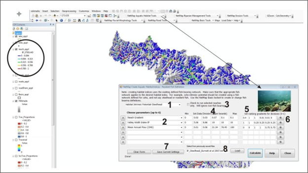 Figure 1. NetMap’s Create Habitat tool is used to build customized aquatic habitat indices, including habitat intrinsic potential (species specific), biological hotspots, and habitat sensitivity, etc. A user selects the type of analysis (1) that will assign that name to the new field in FieldMap for later retrieval by a map generator (or analysis by other tools). Up to six parameters are chosen (2); model can be applied to only a subset of selected reaches (3); the range of values and equal divisions are automatically displayed (4), and the divisions can be adjusted (5). The user determines the variation in weighting assigned to each data division (5), e.g., 0 to 1. The preference curves can be viewed (6). Settings can be saved (7) for later access. Published default models for coho, steelhead and Chinook (Burnett et al. 2007) can be loaded (8).
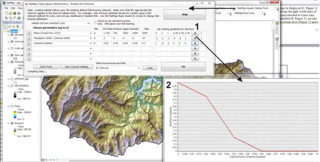 Figure 2. NetMap’s Habitat Creator tool allows the user to quickly view the weighting scores assigned to individual parameters. For example, the weighting function shown for channel gradient indicates that gradients less than 2% produce a higher habitat score compared to gradients greater than 6%. In this example of intrinsic habitat potential for coho juvenile fish (e.g., Burnett et al. 2007), NetMap predicts areas of higher and lower intrinsic potential across the watershed.
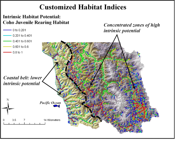 Figure 3. NetMap’s habitat creator tool allows users to examine and visualize the varying spatial distribution of different habitat types (by species) in a watershed. A user can analyze how different landscapes lead to different spatial distributions of habitats. The example shown is from northern California and it shows low habitat potential for coho salmon along the narrow and steep coastal belt of mountains and a much expanded habitat potential in the upper reaches of the Russian River.
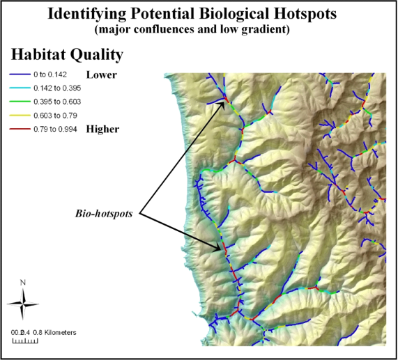 Figure 4. NetMap’s Create Habitat Indices tool is used to predict “biological hotspots”. In this example, hotspots are defined as the convergence of major confluences with low gradient channels with wide floodplains.
A parameter called “habitat sensitivity” can be developed using the same model. Habitat sensitivity can involve channel criteria such as channel gradient, drainage area, and confluence effects (Figure 5). A model based on these and other related channel attributes can indicate those channel segments that are sensitive to influxes of sediment from hillslope erosion, etc. A user can also add hillslope parameters that may relate to the potential for a channel to change its morphology, such as erosion potential (GEP), debris flow potential (at junctions in fish bearing streams), fire risk, burn severity or road density. A user may also create a channel sensitivity index and then use NetMap’s ‘Overlap Tool’ to seFieldh for juxtapositions between risky hillslope conditions and channel sensitivity.
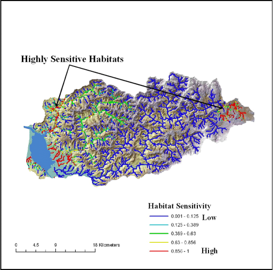 Figure 5. The parameters of channel gradient, floodplain width/channel width, and local sedimentation potential are used to predict habitat sensitivity in the Wilson watershed in Western Oregon.
Although analysts can define their own fish distribution based on local knowledge or their own data, other more general information can be used such as that available from the "streamnet" mapping (for confirmed fish bearing streams). However, the distribution can also be extended beyond that to all streams and rivers that are potential habitats based on gradient and flow thresholds in the intrinsic potential model, including those systems where fish are extinct or extirpated. In this approach, all channels that might have been accessible, but are no longer, are included. For source data, see: http://www.streamnet.org/mapping_apps.cfm
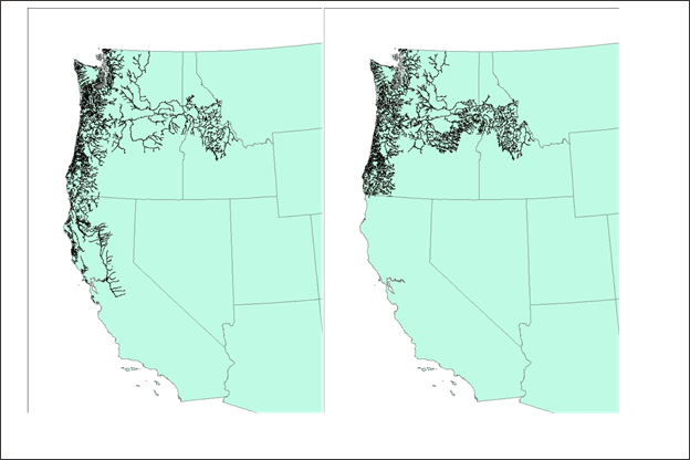 Figure 1. Streamnet distribution in the lower 48 states for coho and Chinook, combined (left panel) and steelhead (right panel).
The contents of Intrinsic Potential (Anadromous) |