| < Previous page | Next page > |
Road Erosion (WEPP)Road Surface Erosion (WEPP)
Parameter Description: The susceptibility of roads to surface erosion (and sediment delivery to streams) according to the WEPP road surface erosion model. For additional information about WEPP technology, see http://forest.moscowfsl.wsu.edu/fswepp/docs/fsweppdoc.html. We gratefully acknowledge Dr. William Elliot of the U.S. Forest Service Rocky Mountain Research Station for assistance is integrating the WEPP road surface erosion model into NetMap. See Figure 3 for information on use of tool.
Data Type: Stream layer, road layer
Field Name: RddWEPP_Rd; Common name: roadWEPP sediment production (road shapefile)
Field Name: RddWEPP_Yd; Common name: roadWEPP sediment delivered to streams (road shapefile)
Field Name: RdWEPP_Yld; Common name: roadWEPP sediment - in reaches (reach shapefile)
Field Name: RdWEPP_Cum; Common name: roadWEPP sediment - in reaches - summed (reach shapefile)
Field Name: RdWEPPSum; Common name: roadWEPP sediment production-summed (orig roads) (original road layer)
Field Name: RdWEPPDSum; Common name: roadWEPP sediment delivery-summed (orig roads) (original road layer)
Field Name: RdWEPPPav; Common name: roadWEPP sediment production-per meter (orig roads) (original road layer)
Field Name: RdWEPPDav; Common name: roadWEPP sediment deliver-per meter (orig roads) (original road layer)
Units: tons/yr
NetMap Module/Tool: Erosion Processes/Road Surface Erosion
Model Description:
The WEPP road surface erosion model is used within NetMap; refer to (http://forest.moscowfsl.wsu.edu/fswepp/) for additional information. The road network (lines) is first broken at pixel cell boundaries (Figure 1). The individual, approximately pixel scale road cells, are then re-aggregated into hydrologically connected segments (tens to a hundreds of meters in length) that represent water flow paths from high (topographic) points to low (pour) points or to defined streams. These hydrological road segments can be viewed in terms of their drainage diversion potential. For example, in the absence of secondary road drainage structures, the drainage diversion road segments should indicate the water diversion potential of any road segment, particularly under conditions such as during large storms or following wildfires. Refer to NetMap’s Road Drainage Diversion Potential parameter.
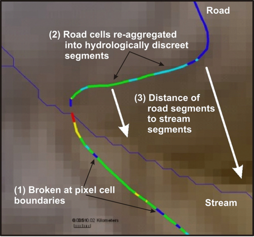 Figure 1. In NetMap, road layers (lines) that may be kilometers long are broken at pixel cell boundaries (1). They are then re-aggregated into hydrologically discreet segments between topographic high and low (pour) points using NetMap's road drainage tool. These segments are used in the WEPP road surface erosion model. In addition, each road segment is linked (by distance and hillslope gradient) to the nearest downslope channel segment, called the “buffer” in WEPP, that influences the potential for road sediment to enter streams.
Surface erosion on roads is governed by road gradient, length of road that is hydrologically connected (e.g., length of overland flow on a road surface), road width, road surfacing (native, gravel), traffic level (high to low), and time since grading (Luce and Black 1999, Sugden and Woods 2007). The WEPP road surface erosion model (Elliot et al. 1995, http://forest.moscowfsl.wsu.edu/fswepp/docs/wepproaddoc.html) employs the parameters of road width, drainage length, road gradient, surface material, soil type and traffic level. Since WEPP predicts sediment delivery to streams (t/yr), the intervening hillslope distance (and gradient) between individual road segments and the nearest stream influences the amount of sediment delivered to channels. If the road drains directly to a stream channel, no buffer is considered.
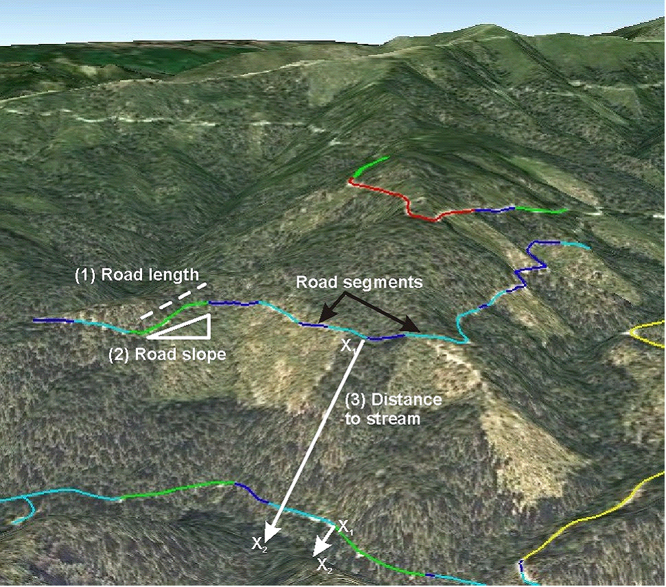 Figure 2. Important factors of road surface erosion include road segment length (1) that is hydrologically distinct (shown by the different color codes, the slope of the road (2), and the distance of individual road segments (drain or pour points) from individual stream segments (3). A simple index or proxy of road surface erosion (Road Erosion Index tool) uses these three parameters.
To use the WEPP tool to make predictions about road surface erosion potential (tons/yr) requires additional, site specific information on climate (a sequence of storms over decades). Climate data can be quickly obtained from CLIGEN.
Note, before running WEPP, a user must first determine road drainage connectivity, using the Drainage Diversion Tool.
The objective of the NetMap analysis of road surface erosion is to identify road segments that have a high likelihood of producing large amounts of fine sediment and delivering that sediment to high value streams and fish habitat. Road surface erosion can be reduced by increasing the number or frequency of cross drains (thereby reducing the effective length of overland flow on a road surface) and improving road surface materials (such as placement of gravel on a native soil surface). Reducing road surface erosion can be reduced by placement of rolling dips and other secondary drainage structures such as ‘open tops” (Figure 3). Continuing road maintenance can be expensive and in recent years resource managers have seen budgets severely limit their capacity for that work. In some cases managers are abandoning, storing, or decommissioning roads in efforts to remove their long-term impacts in critically important areas. Because road restoration, including obliteration and recontouring, also can be very expensive (though it does limit long term maintenance) it is increasingly important to be able to focus limited restoration funds where they can be most useful.
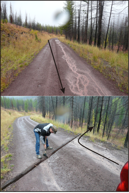 Figure 3. (Top) Long stretches of road can be hydrologically connected, via overland flow. In the Clearwater River basin that can lead to considerable surface erosion and the delivery of both fine sediments and other materials (nutrients) to streams. (Bottom) The use of cross drains (a form called ‘open tops’ in the photo) can be used to decrease the length of overland flow and thus decrease the amount of surface erosion and the volume of sediment and other materials reaching stream channels. Arrows illustrate the accumulation of flow and its disruption due to the cross drain, during conditions of light rain.
Running NetMap's WEPP Road Surface Erosion Tool
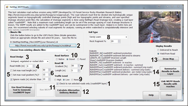 Figure 4. NetMap’s road surface erosion model (WEPP) contains a series of required parameters including: (1) the selection of a set of road segments (from the Road WEPP layer, which is comprised of hydrologically discreet segments [Figure 1] and see Tool for calculating it); (2) use of 50-year climate from CliGen; (3) information on road design, including road width (4); (5) ignore road segments of a minimum length (optional); (6) set maximum road gradient (an option, see Figure 5), (7) set road fill gradient and length; (8) select soil type; and (9) select traffic level and road surface type (10). (11) Run the tool (it is recommended to run only small subsections of roads, since running WEPP on an entire NetMap digital watershed datasets could be very time consuming [e.g., run it over night]). (12) Use an alternative sediment delivery to streams approach, a conservation of mass method (see here). (13) Two different outputs can be displayed. (14) Results can be summarized to the original road layer, road segment IDs and (15) Road WEPP results can be linked to stream segments (reaches).
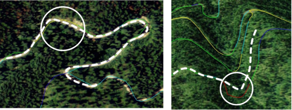 Figure 5. Colored lines represent GIS roads draped onto a Google Earth image in the northeastern corner of the Clearwater basin. Dashed white line overlays upon exact road locations on the satellite imagery. Road misalignments are highlighted by the circles. Exaggerated road gradients (considerably in excess of 12%) can lead to exaggerated road surface erosion predictions using WEPP. In NetMap’s WEPP tool, a user can specify a maximum road gradient to reduce some of the road gradient error due to misalignment problems (Figure 4, #6). Ideally it is important to verify the correct alignment of roads in a GIS and correspondingly on the DEM so that the most accurate predictions of road surface erosion can be produced in NetMap. In addition, road layers should be updated to reflect the most current status of the road use (active, decommissioned, storage). Another potential problem is that some of the roads contained within the GIS layer used in this analysis are already decommissioned but are not indicated as such in the GIS road layer.
Technical Background:
Example Application and Use:
The application of NetMap in the Clearwater River watershed of western Montana (1016 km2, 250,000 acres) represents a demonstration analysis of how the NetMap community science system can be applied to restoration planning. Funded by the South West Crown Collaborative Forest Landscale Restoration Project (CFLR) and the Clearwater Resource Council (CRC), this NetMap application utilized a 10-meter digital elevation model, a road layer provided by the Ecosystem Management ReseFieldh Institute (EMRI), information on fire risk, watershed function and anticipated habitat condition from the Lolo Forest (USFS) and distribution of cutthroat and bull trout by Montana Fish Wildlife and Parks (MTFWP) to explore the potential utility in road related restoration and conservation management.
The objective of this analysis is to evaluate the road network in the Clearwater basin in support of restoration planning to demonstrate a process of prioritization for: 1) improving road drainage and reducing surface erosion to valuable stream habitat (e.g., high quality fish habitat); 2) improving fish passage at road crossings; 3) stratifying roads for effectiveness monitoring; and 4) extrapolating and/or forecasting basin wide effects of road restoration programs.
Step 1: Map the distribution and values of streams and fish habitat
The MTFWP has identified the distribution of cutthroat trout and bull trout in the Clearwater basin and developed habitat ranking scores for each (Fig. 7). The GIS layers were imported into NetMap and the habitat value for cutthroat (1-10) and for bull trout (1-10) were combined to create a composite index of habitat suitability (Figure 8).
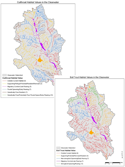 Figure 7. Habitat distribution and values for cutthroat and bull trout in the Clearwater basin (source: MTFWP; Rieman et al., 2012).
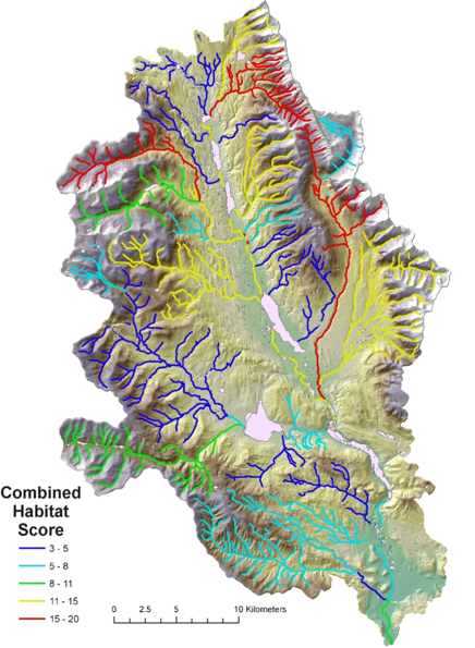 Figure 8. The stream habitat values for cutthroat and bull trout (Fig. 2) were combined into a composite score for use in NetMap.
Step 2: Analyze road drainage diversion potential.
To predict road surface erosion using WEPP requires knowledge of the hydrologic connectivity of roads or the potential length of overland flow on roads (e.g., Fig. 1). Typically, GIS road layers contain road segments that are kilometers long and are not delineated by specific physical attributes. Thus, in NetMap, GIS road layers are first broken at pixel cell boundaries thereby creating a linked population of road segments of approximately 10 m in length (when using a 10-m DEM). Next, road overland flow directions are determined for each small road segment (based on road gradient and orientation) and the small road segments are re-aggregated to create hydrologically connected road segments based on hillslope topography . In other words, road drainage (pour) points are determined based on topographic highs (ridges) and lows (swales) and further constrained by roads intersections with stream channels (in this analysis all road-stream crossings are assumed to have functioning drainage structures [bridges, culverts]). In the current version of WEPP in NetMap, secondary drainage structures are not included in the analysis, although a user can set a fixed flow accumulation distance in the tool (for example, if the user knows that a specific stretch of road has secondary road drainage structures [Fig. 1] every 400 feet, they can specify that constraint when running the tool). Road hydrologic connectivity at the scale of the entire watershed is predicted to range between 10 and 2500 m (Fig. 4).
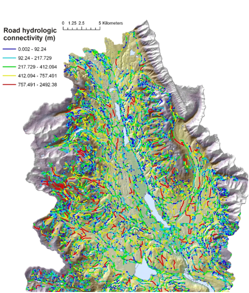 Figure 9. Predicted road hydrologic connectivity ranged between ten and 2500 meters (average 133 m). This parameter, during large storms or following fires when secondary drainage structures may be compromised, could be viewed as an index of ‘road drainage diversion potential’. The drainage diversion index could be used to identify locations where field crews could check on drainage efficacy during or after storms or following fires.
Step 3: Analyze road surface erosion potential, point sources to streams.
The WEPP road analysis tool in NetMap can be run at any spatial scale, ranging from a single road segment (average 130 m in the present analysis) to the entire watershed encompassing 16,418 individual segments. In this demonstration analysis, WEPP was run across the entire road network in the Clearwater basin.
The following parameters were used in WEPP within NetMap: a) road hydrologic connectivity (Fig. 9); b) climate, using Seeley Lake (in the Clearwater basin) [obtained from WEPP’s stochastic climate generator, Cligen]); c) road width = 4 m; d) native rock surfacing (personal communication Shane Hendrickson, U.S.F.S., Lolo National Forest); e) high traffic (assumed constant); f) inslope, vegetated and rocked ditch; g) fill gradient and slope of 50% and 5 m; h) soil type sandy loam and i) hillslope buffer length and slope (e.g., the hillslope located between individual road segments and channels) determined for each road segment (ave. 130 m) using NetMap’s analytical capabilities. Users can change these parameter settings in subsequent runs of the model within NetMap.
Predicted annual road surface erosion ranged from near zero to 4.7 t (metric tons, 1000 kg) per year. The average predicted erosion to streams was 0.04 t/yr with a standard deviation of 0.13 t/yr (Fig. 10). The road segments (total 16,418) with the highest predicted sediment yields to streams having some combination of long road segments that are hydrologically connected (Fig. 9, e.g., several hundred meters plus), steeper gradients, and close proximity to channels (limited buffers).
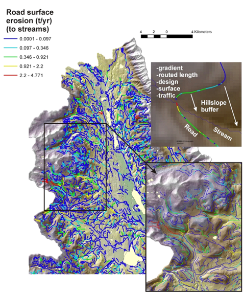 Figure 10. Road surface erosion (as delivered to streams) in the Clearwater basin ranged from very low (near zero) to a maximum of 4.7 tons/year. In the figure, individual road segments are color coded according to predicted annual sediment yield. Predicted sediment yields to streams are sensitive to the hillslope distance and gradient (e.g., buffer) from individual road segments to streams, as illustrated in the figure (upper right).
|