Thermal Energy Sensitivity

Thermal (Radiation) Energy to Streams: Sensitivity Analysis

Parameter Description: This tool evaluates effects of different riparian buffer strategies on changes to thermal loading due to changes in riparian vegetation cover. The tool can perform a sensitivity analysis of the thermal load changes (with and without vegetation) to determine where the most thermally at risk streams are located in a watershed, a useful analysis when considering the effects of wildfire or timber harvest. Thermal loading (watt-hours/m²) to streams governed by channel width and orientation, topographic shading, vegetation shading, and location and date. Parameters include: 1) solar radiation-vegetated, 2) solar radiation-bare earth, and 3) solar radiation difference: vegetated minus bare earth.

NetMap presently does not contain a stream temperature model because of the site specific nature of the empirical calibration needed (water temperature) that is needed to make accurate stream temperature predictions. NetMap’s thermal load tool can inform stream temperature models.

Data Type: Line (stream layer)

Field Name: SolVeg; Common Name: Vegetated solar radiation

Field Name: SolBare; Common Name: Bare Earth Solar Radiation

Field Name: SolDif; Common Name: Solar radiation difference (vegetated – bare)

Units: Watt-hours/m²

NetMap Module/Tool: Vegetation/Fire/Climate - Thermal Load

Model Description:

NetMap’s thermal loading tool (NTLT) focuses on a suite of vegetative and topographic factors that control the relative potential for stream warming in watersheds at the river network scale. NTLT focuses on thermal loading, rather than predicting stream temperatures, since accurately predicting stream temperatures requires considerable site-specific calibration (using water temperatures, see http://www.fort.usgs.gov/products/software/SNTEMP/) and because predicting stream temperatures accurately requires site-specific information on factors such as groundwater flow, channel substrate conditions and hyphoreic flow.

NTLT’s prediction of thermal loading uses the parameters of direct beam and diffuse solar radiation with respect to 1) topographic shading, 2) channel width, 3) aspect, 4) latitude, and 5) streamside vegetation height and density. NTLT uses FieldMap’s Solar Radiation tool and it calculates incoming solar radiation for every vertex in the stream network (each stream segment may have numerous vertices based on a channel’s path across pixels). FieldMap’s solar radiation model uses hourly intervals on July 20, typically the hottest day of the year. Incoming diffuse, direct, and total radiation values are computed for every hour, with the bare-earth DEM providing topographic shading. Thermal energy (watt-hours/m²) is calculated as an average of all intersecting vertices for each reach summed over the daylight period.

Referencing Figure 1, an analyst can specify the dimensions (forest width, tree height, vegetation density) of two spatially coincident vegetation types (1 and 2, the ‘riparian buffer forest’ and the ‘outer forest’ in case there is a management scenario in which the vegetation density is different between them [note, tree height needs to be the same]). The tool can be run on only a selection of reaches (3) using FieldMap’s selection tool or the entire basin can be analyzed (all streams, fish and non fish bearing) (Figure 1). Note that running the entire basin that is comprised of thousands of stream segments may require considerable time (more than a day)! Thus, it may be best to only run selected reaches of particular interest. Or, only the fish bearing network could be selected at the scale of a watershed. If only a portion of the network is selected and run, and then, at a later date, another portion of the network is analyzed, a user can set the previous selected reach values to zero, for purposes of uncluttering map displays (4). In addition, selected reaches can be saved and or reloaded for subsequent analyses (4). The map generator (5) contains three map options: 1) total bare earth radiation, 2)total radiation with vegetation (including buffer conditions), and 3) difference between bare earth and vegetation.

Running the temperature model at the basin scale can provide watershed-level screening information on where thermal loading increases may be the highest.

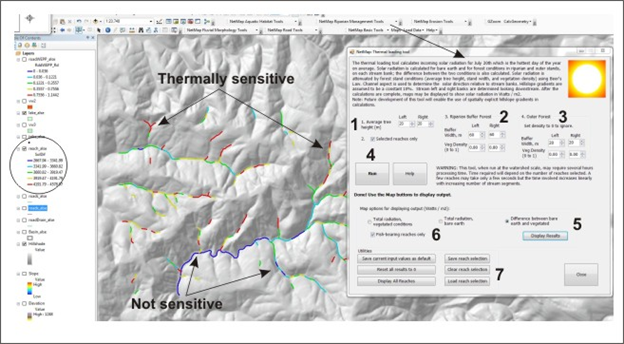Figure 1. The NTLT’s graphical user interface allows a user to specify up to two (adjacent) buffer dimensions and characteristics (e.g., width, vegetation height, vegetation density) (1) A user selects an average tree height on both sides of the channel, for both the inner and outer buffer (same for both), (2 & 3) The user selects the appropriate buffer width and vegetation density (0-1) (e.g., canopy cover, canopy closure, leaf area index, see http://www.netmaptools.org/Pages/links/Assessing_canopies.pdf ; http://www.netmaptools.org/Pages/links/LIA_beerslaw.pdf; http://www.netmaptools.org/Pages/links/Ringold_etal_2003_JAWRA.pdf ). The analysis can be limited to one buffer (2). (4) The tool is run; it is recommended that only subsets of reaches are selected, running an entire standard NetMap dataset could take an hour or more. (5) The type of output is selected including bare earth, vegetation conditions, and the difference between them (a sensitivity analysis). (6) The display can be done only for fish bearing streams. (7) There are a number of utilities.

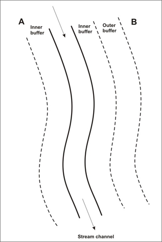Figure 2. A thermal analysis can utilize either a single buffer (A) or a double buffer (inner, outer) shown in B.

Sensitivity Analysis

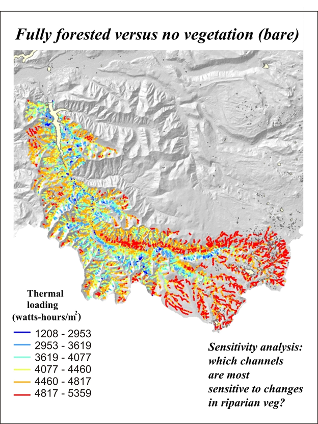Figure 3. NetMap's thermal tool is used to calculate a sensitivity analysis - which channels, if riparian vegetation was removed or decreased, would be the most sensitive. In watt-hours/m².

Figure 4. NetMap's thermal tool is sensitive to varying vegetation density. The width of the buffer required to meet a specific thermal loading target increases with decreasing vegetation density. See also Figures 5 through 7. In watt-hours/m².

The numerous factors involved with predicting thermal loading or thermal sensitivity of individual streams (latitude, time of year, topographic shading, stream orientation, channel width, and vegetation height, width and density. It is informative to do a sensitivity analysis to observe how certain factors govern radiation loading. If we keep latitude, time of year (August), stream orientation (N-S), and channel width (10 m) constant, we can examine how vegetation height, buffer width and vegetation density affect thermal loading (these variables are important from a riparian management perspective, specifically the design and management of riparian forests, including buffer strips. See sensitivity analysis in Figures 5 through 7 below.

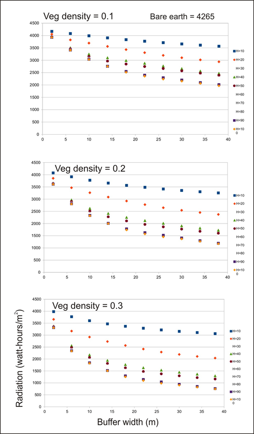Figure 5. A sensitivity analysis for a N-S trending channel of 11 m wide during August in southern coastal Oregon. Note the effects of buffer width, tree height and vegetation density on radiation loading. Note the bare earth (no vegetation) radiation loading of 4265 watt-hours/m². Note that the effects of tree height increase with increasing vegetation density and that the effects of tree height begin diminishing with trees greater than about 30 to 40 m.

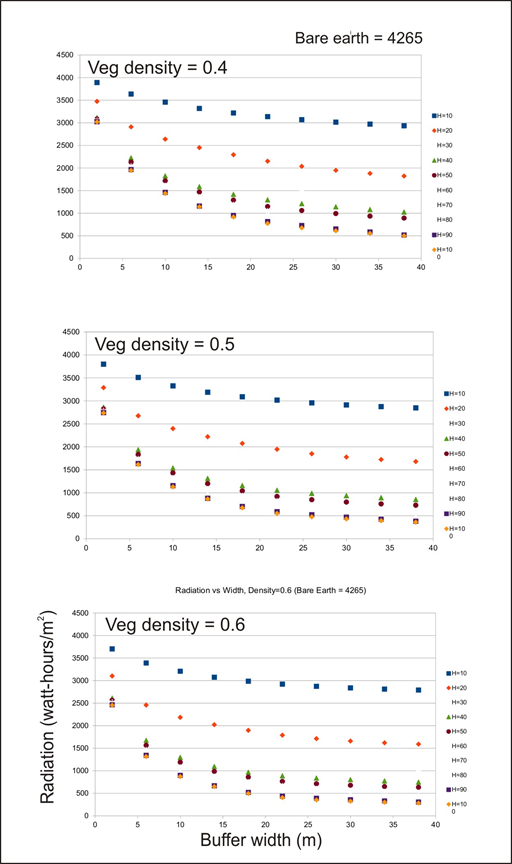Figure 6. A sensitivity analysis for a N-S trending channel of 11 m wide during August in southern coastal Oregon. Note the effects of buffer width, tree height and vegetation density on radiation loading. Note the bare earth (no vegetation) radiation loading of 4265 watt-hours/m². Note that the effect of buffer width are effected by vegetation density. As density increases, the effect of buffer width on decreasing radiation becomes muted.

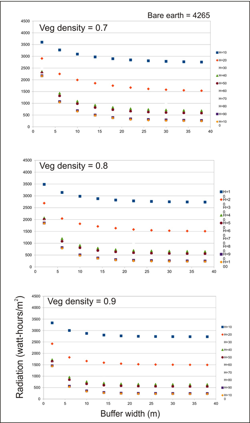Figure 7. A sensitivity analysis for a N-S trending channel of 11 m wide during August in southern coastal Oregon. Note the effects of buffer width, tree height and vegetation density on radiation loading. Note the bare earth (no vegetation) radiation loading of 4265 watt-hours/m². Note that at very high vegetation densities, the effective buffer width ranges from 15 to 30 meters.

Technical Background:

The prediction of thermal loading uses the parameters of direct beam and diffuse solar radiation and includes the factors of 1) topographic shading, 2) channel width, 3) aspect, 4) latitude, and 5) streamside vegetation height and density. NTLT uses FieldMap’s Solar Radiation tool and it calculates incoming solar radiation for every vertex in the stream network (each stream segment may have numerous vertices based on a channel’s path across pixels). FieldMap’s solar radiation model uses hourly intervals on July 20, typically the hottest day of the year. Incoming diffuse, direct, and total radiation values are computed for every hour, with the bare-earth DEM providing topographic shading. Thermal energy (watt-hours/m²) is calculated as an average of all intersecting vertices for each reach summed over the daylight period.

Direct Beam Radiation:

NTLT computes the direct radiation for each hour for the DEM (Figure 8). The user supplies vegetation conditions, including height, width (buffer) and canopy density (0-100%). With the user-supplied vegetation conditions, the bare-earth radiation is diminished using light attenuation through the canopy (using Beer’s Law, Monteith and Unsworth 1990).

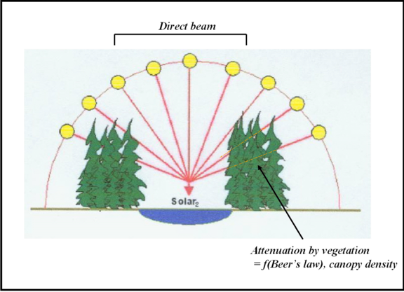Figure 8. NetMap’s thermal input tool computes the incoming direct beam radiation throughout the hottest day of the year (July 20^th), attenuated by streamside vegetation (using Beer’s Law), and sums those values for each stream segment. Figure from Boyd and Kasper (2003, 2007).

If the shadow length spans or is greater than the stream width, the channel is shaded. If shadow length is narrower than the channel width, then some portion of the channel is receiving direct beam radiation. Another portion may be traveling through streamside vegetation although light would be attenuated. It is important to calculate the solar path length through the streamside vegetation (Figure 9).

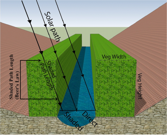Figure 9. Thermal loading to the stream (watt-hours/m²) is affected by the solar azimuth, stream azimuth and solar altitude as well as vegetation shading. Figure modified from Boyd and Kasper (2003, 2007.

The direct beam radiation that travels through the forest canopy (or buffer canopy) is calculated as follows (Figure 9). The path length (P) is:

P = buffer width/COS (SA * Pi/180 degrees)

Where SA is the solar altitude (Figure 4). The shade density (SD) is:

1-Exp (Log (1-VD)/10) * P

where VD is vegetation density (VD) that could be estimated using canopy closure (Jennings et al. 1999).

Thus, direct beam radiation (DB) through the canopy (DBR) is:

DBR = DB * (1 – SD)

The calculation of direct beam radiation must also account for the relationship between solar altitude, stream orientation and path length (not shown). The needles and leaves are assumed to be perfect radiators and thus NTLT ignores scattering within the canopy.

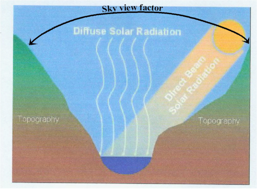Figure 10. NetMap’s thermal tool assumes streamside vegetation is rectangular in shape with a height, width and vegetation density. Sunlight passing through streamside vegetation is attenuated by Beer’s Law.

The shaded portion of the stream is divided into two portions – that which receives sunlight through a portion of the canopy, and that which receives sunlight through the full width of the canopy (generally only very early or late in the day). For each of these portions, we calculate an average path length of the sunlight through the canopy. The bare earth radiation is attenuated using the shade factor and path length (using Beer’s Law), and applied to the affected channel surface area (Figure 11).

Figure 11. A sketch showing the geometry of light transmission to a stream including unobstructed direct incident radiation and light attenuated through a vegetative zone or buffer. The path length through the vegetation is a function of vegetation or buffer width, stream aspect, solar altitude and solar azimuth. Attenuation follows the principles embodied in Beer’s Law (Oke 1978).

For each hourly interval, NTLT computes the incident angle of the sun and the channel, using the sun elevation (solar altitude), and the difference between the sun azimuth and the channel azimuth. NTLT then analyzes the resulting solar path length and determines how much of the channel is receiving direct, non-shaded sunlight, and how much of the channel is receiving attenuated sunlight; this is also influenced by channel width. NTLT does not consider overhanging vegetation and the vegetation is assumed to be represented by a vertical wall adjacent to the channel. NTLT considers the vegetation buffer to be a rectangular (cross-section) feature, which does not climb up adjacent hillsides. This is a known limitation of the model, which tends to cause an overestimation of incoming radiation. In future versions of NTLT, the hillslope angle and the change in vegetation canopy will be addressed.

Diffuse radiation:

NTLT computes the diffuse radiation for each hour for a flat-surface DEM (sky view factor of 1). For each stream segment, NTLT calculates a sky view factor based on the topography, channel width, length, and vegetation height, assuming that the vegetation is blocking the sky at either end of the channel as well as both sides (e.g., Figures 12). The bare earths diffuse radiation value for each hour is multiplied by the sky view factor, and the hourly values are summed to get the total daily diffuse radiation value.

Figure 12. The solar components controlling thermal loading to streams include direct beam solar and diffuse solar radiation. Figure modified from Boyd and Kasper 2003, 2007.

Total Radiation:

Total radiation is the sum of direct and diffuse radiation. In watt-hours/m².

How NTLT works:

NTLT considers three different forest conditions for each run of the tool: 1) bare earth, 2) existing or fully forested, and 3) a stream buffer. Parameters that describe vegetation include width, height, and vegetation density (0 – 1 and analogous to canopy closure but see Jennings et al. 1999) (see: http://www.netmaptools.org/Pages/links/Assessing_canopies.pdf ; http://www.netmaptools.org/Pages/links/LIA_beerslaw.pdf; http://www.netmaptools.org/Pages/links/Ringold_etal_2003_JAWRA.pdf ). Initial condition generally refers to a more heavily vegetated condition, while buffered condition generally refers to a less-vegetated condition (i.e. shorter trees, smaller width, and lower vegetation density). Incoming solar radiation, summed over each hourly interval, is computed for bare earth, existing or fully forested conditions. Thermal loading is reported in units of watt-hours per square meter.

The three map outputs include total bare earth radiation, radiation under vegetated conditions (can include buffers), and the difference between bare earth and vegetated (Figure 10). The bare earth radiation parameter is useful to see intrinsic thermal loading to streams. The difference between forested and no vegetation parameter provides a sensitivity analysis of the intrinsic sensitivity to removal of vegetation such as following timber harvest or wildfire (Figure 7). The difference between existing conditions and buffered parameter provides information about how effective buffers of specified dimensions are in protection streams from thermal loading.

In the attribute table the field names of the parameters are:

SolVeg = solar radiation, vegetated

SolBare = bare earth solar radiation

SolDif = solar radiation difference

Made with help of Dr.Explain