| < Previous page | Next page > |
|
Tongass National Forest Channel Classification System
 1.0 Overview
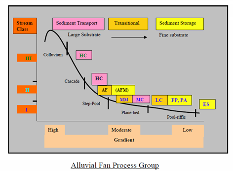
Steve Paustian designed and applied a stream classification system for the Tongass National Forest in southeast Alaska based primarily on aerial photography to support watershed management (Paustian et al. 1983). The method was updated in 2010 to further differentiate channel types based on secondary characteristics such as channel width, incision depth, gradient and channel pattern (Channel Type User Guide Revision 2010). The Tongass classification system is based on three hierarchical morphometric groupings: 1) Process group, 2) Channel type and 3) Channel type phase (Figure 1). There are seven process groups: i) alluvial fan, ii) estuarine, iii) floodplain, iv) glacial outwash, v) high-gradient contained, vi) low-gradient contained, vii) moderate-gradient contained, viii) moderate gradient, mixed control and ix) palustrine. There are three channel type criteria: i) channel width, ii) channel gradient and iii) incision depth (Figure 2). Channel type phase include smaller-scale channel features such as step-pool morphology, bedrock gorge and streamside vegetation characteristics.
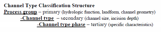 Figure 1. Tongass channel classification is based on three morphometric groupings. 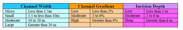 Figure 2. Revised (2010) channel type groups, including differentiating among large, moderate, small and micro. From Channel Type User Guide Revision 2010. The NetMap-based Tongass channel classification system, that relies on remote sensing data only (digital elevation models and GIS maps), uses process groups and channel types. The channel type phase is not included, but could be added based on field observations, and advances in remote sensing technology using LiDAR DEMs (which partially cover southeast Alaska, as of 2020).
2.0 NetMap Tongass Channel Classification Program
In late 2019 through early 2020, Terrainworks built a computer program, within the NetMap system of virtual watersheds, to replicate the Tongass channel classification application using only remote-sensing information, including LiDAR and IfSAR DEMs (1-2 m and 5 m respectively) and GIS data pertaining to glacial extent, coastal morphology and vegetation characteristics. This required development of two new mapping tools. (1) Channels within alluvial fan landforms are identified to account for the alluvial fan process group (Figure 3) and (2) The depth of channel incision into the surrounding terrain is estimated (Figure 4).
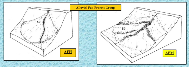 Figure 3. Sketches of alluvial fans, typical of southeast Alaska. From Channel Type User Guide Revision 2010. 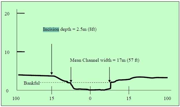 Figure 4. An example of "incision depth". Note the difference with bankfull channel depth. From Channel Type User Guide Revision 2010. To identify channels within alluvial fans, a morphometric rule set was developed that contained: 1) an upstream source of sediment using NetMap's GEP attribute (summed and GEP per unit area) as a proxy for sediment supply, 2) gradient range typical of fan landforms, 3) distinct upslope gradient break at fan apex and another at the distal end (optional), 4) general lack of incision over the body of the fan, 5) a convex-up landform shape based on NetMap's horizontal and plan curvature attributes and 6) landscape position (where a channel node falls between the valley floor and ridge top, calculated as a raster).
For LiDAR DEMs, the initial set of thresholds include: i) upstream gradient < 0.20, downstream gradient > 0.03; ii) GEP cumulative > 4,000, GEP per unit area > 0.01; iii) channel incision depth < 2.5 m; iv) plan curvature < 1 and v) landform position > 0.0175 and <0.34. These reflect topographic conditions where channels have: an upslope source of sediment; are not confined within a valley; are located near the base of hillslopes; have appropriate alluvial fan gradient range; and are located on concave down landforms. For IfSAR 5m DEMs, the only difference is GEP cumulative > 800, GEP per unit area > 0.005. All of these thresholds can be adjusted.
Channels located on alluvial fans are shown in Figure 5. Most locations appear appropriate; the left-side of the valley shows a series of fan channels on a set of interdigitated fans, commonly referred to as bahadas. Some of the fan channels on the right-side of the valley are located in broader depositional areas.
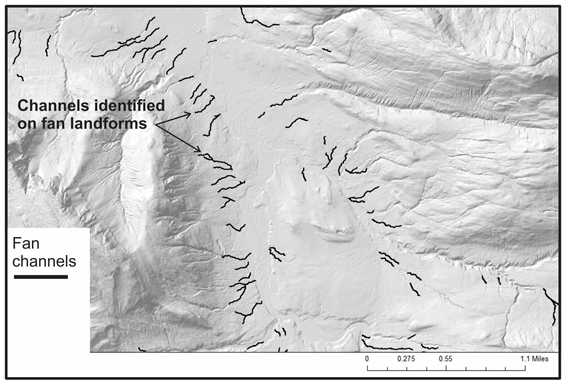 Figure 5. Channels identified on alluvial fans based on 2-m LiDAR DEMs on the North Chichigof Island. The depth of incision program fits a smooth surface to channel-adjacent topography, centered along each channel node. A circular window of a specified radius (in terms of number of channel widths) is fitted with a quadratic surface to all DEM points within that window (to determine best fitting surface). DEM points within a specified distance (also in terms of channel widths) are not considered, to exclude morphology, like channel depth. For small channels (generally < 1 m wide), a minimum radius is specified to include sufficient terrain (DEM cells) to define the surface. For larger channels, the window may become too large and extend beyond local floodplains, thus a maximum radius controls the lateral extent of the circular window. The depth of incision into the stream-adjacent terrain is the difference between the actual channel nodes and the fitted surface. The predicted depth of incision of channels in the North Chichigof Island area using 2-m LiDAR is shown in Figure 6.
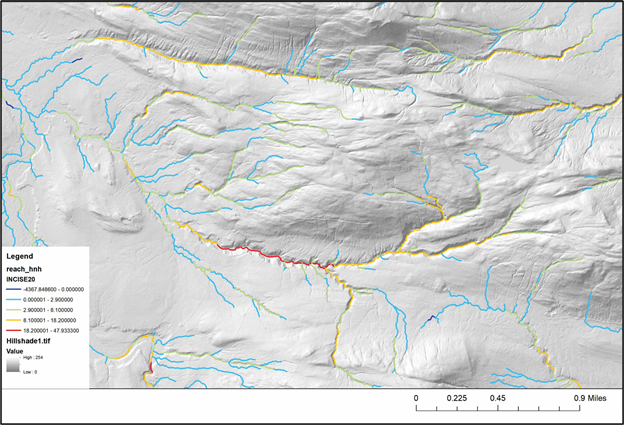 Figure 6. Predicted channel incision values (m) for an area in North Chichigof Island using 2-m LiDAR DEMs. Many of the fan channels shown in Figure 5 have corresponding low incision values. Deeply incised canyon reaches are identified.
Other GIS layers provided by the Tongass National Forest included palustrine areas (muskeg) and coastal zones to identify estuary areas (below mean high, high water) (Figure 7).
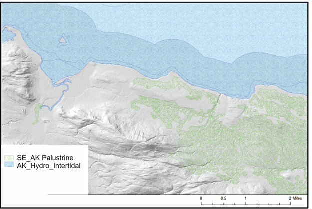 Figure 7. Tongass National Forest GIS layers for palustrine and intertidal environments.
The uplifted estuary beach channel classification relied on Larsen et al. (2002) reconstructed rates of uplift reveal significant spatial variability across southeast Alaska (Figure 8).
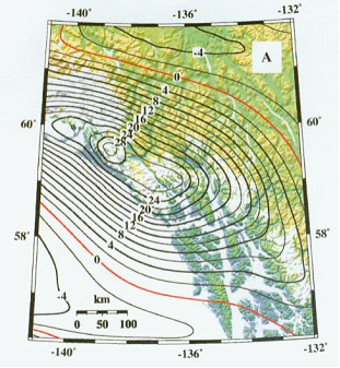 Figure 8. Reconstructed rates of uplift from isostatic rebound across southeast Alaska (Larsen et al. 2002).
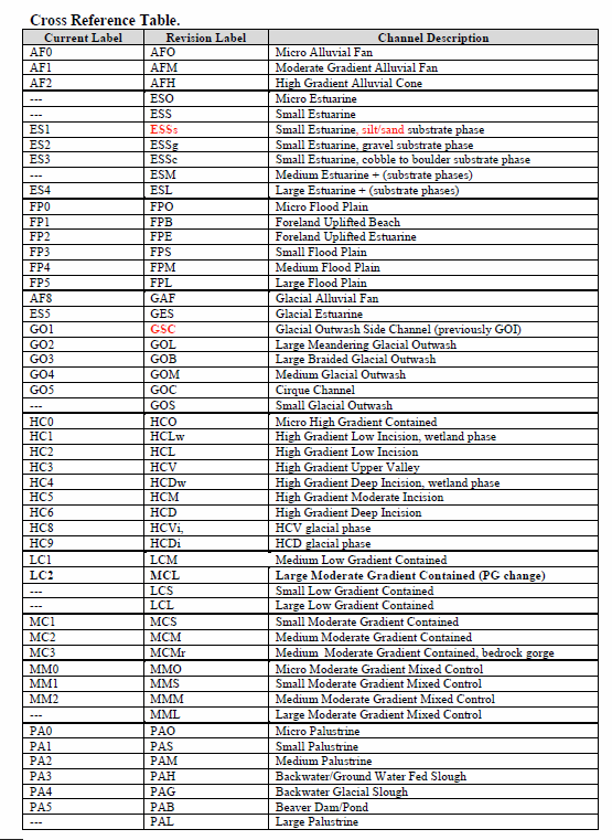
NetMap's Tongass channel classification system as represented in the remote sensing model is outlined in Table 1. Landform classes, channel types (by code), channel bankfull width, gradient, incision and floodplain width are included. Refer to the Channel Type User Guide (Revision 2010) for further information on channel types indexed by code (AFO etc.).
Table 1. Channel classification criteria and the resulting types within NetMap's remote sensing based Tongass Channel Classification system. Table entries by Lee Benda and Emil Tucker (2020).
A refers to 2010 classification update. B refers to original 1992 classes.
Table 2. Channel classification labels (original 1992 and updated 2010) and the associated channel descriptions (from Channel Type User Guide Revision 2010). The revision labels are used in the NetMap remote-sensing based channel classification in the Figures below.
 The model flow chart that governs how the various attributes are combined, using thresholds identified in Table 1, to create distinct channel classes within NetMap (Figure 9).
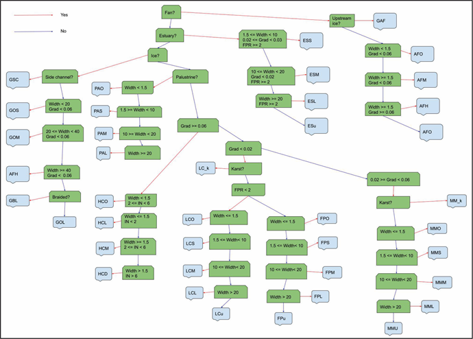 Figure 9. Flow chart of model pathways that shows morphometric attributes, their threshold values and how selections were made in the NetMap Tongass channel classification system. Channel class labels are located in Table 2.
The remote-sensing based model was applied as a pilot in the North Chichigof Island using 2-m LiDAR DEMs and IfSAR 5 m DEMs. NetMap's virtual watershed datasets were available with both DEM resolutions. The LiDAR based model predictions of channel classes is shown in Figures 10 through 11. Channel class labels are located in Table 2.
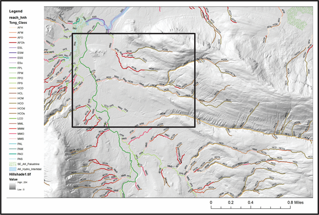 Figure 10. NetMap's Tongass channel classification in North Chichigof Island. The box shows the area contained within Figure 11.
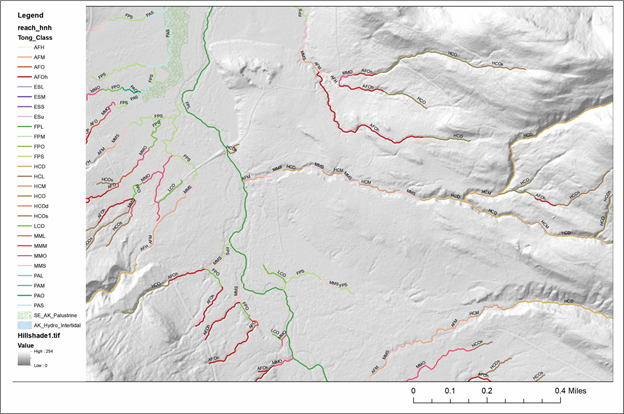 Figure 11. NetMap's Tongass channel classification in North Chichigof Island. Channel class labels are located in Table 2.
The remote-sensing based channel classification system is currently in review by the Tongass National Forest (spring, 2020). Future modifications are likely. The Tongass channel classification system can be applied across southeast Alaska using NetMap's virtual watersheds (LiDAR and IfSAR based).
References
Channel Type User Guide Revision (2010).
Larsen, C.F.; Motyka, R.J.; Freymueller, J.T.; Echelmeyer, K.A.; and Ivins, E.R. (2005). Rapid Viscoelastic uplift in southeast Alaska caused by post-Little Ice Age glacial retreat Earth and Planetary Science Letters (EPSL) Volume:237, p 548-560, Elsevier.
Paustian, S.J.; Marlon D.A.; Kelllher, D.F. (1983). Stream channel classification using large scale aerial photography for southeast Alaska watershed management.
In: Renewable resources management symposium: Applications of remote sensing: [Date of meeting unknown]; [Location of meeting unknown]. Falls Church, VA:
American Society of Photogrammetry: 670-677.
|