| < Previous page | Next page > |
Reach Scale, Forest GrowthWood Recruitment (Reach Scale)
Parameter Description: The Reach Scale Wood Recruitment Model (RSWM) calculates wood loading and accumulation in a reach based on vegetation mortality (generated in forest growth models or estimated), bank erosion, and decay. The model can be run for one or more years (running multiple years will require input from a forest growth model). The model runs independently of GIS, and can run independently of NetMap.
[Note, NetMap also contains a watershed scale wood recruitment model that can be run using a data on riparian conditions for a single year (e.g., average tree height, diameter, density and mortality rate) or using forest growth model output.]
Data Type:
Input: Stand tables from forest growth models (e.g., FVS, Organon, Zelig)
Output: Tables, plots of wood recruitment over time
Name: Wood recruitment to streams
Units: Number of pieces of wood (100m-1 reach length yr-1) or wood volume (m3 100m-1 reach length yr-1)
NetMap Module/Tool: Vegetation/Fire/Climate/Riparian Management/Reach Scale Wood Recruitment
Model Description: The reach scale wood recruitment model (RSWM) calculates the number of pieces and volume of wood entering a stream reach based on the projections from forest growth models that are stored in stand tables (the model can also be run for a single year). Each record in a stand table contains the year, species, diameter at breast height class (DBH), live trees per area and height, and forest mortality per area and tree height – the latter two by mortality type. Mortality types can be modeled (calculated by a forest growth simulator), and can also include insect, disease, and wind throw. RSWM calculates the probability for each record that any dead trees will fall into the stream reach, at one meter distance increments from the reach. The probability (P) that a tree will fall into the stream depends on the tree’s proximity to the reach, tree height, and the valley side slope (Eq. 1):
 , (Eq. 1) , (Eq. 1)where,
d is the distance to the reach, h is the height of the tree to its point of intersection with the channel, and σ is the empirically derived standard deviation of the fall direction in degrees for the valley side slope gradient (Figure 1). When the distance to the reach is zero, it is assigned to one cm to avoid divide by zero errors. When the valley side slope is less than or equal to 40°, σ = 76; when the valley side slope is greater than 40°, σ = 41 (Table 3; Sobota et al., 2006). The probability is calculated for each of five mortality types as these can have different mortality rates and tree heights.
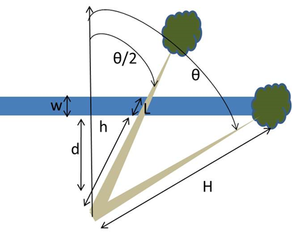 Figure 1. Dimensions used in RSWM equations.
.
The number of pieces of wood in the stream is the probability of tree fall into the reach multiplied by the tree mortality for that mortality type. To classify the piece size, the diameter of the piece is calculated for the middle of the piece and the user can select one of three ways to accomplish this. The diameter of the tree is calculated at 3 places: the near bank (d1), the middle of the piece in the reach (dMid), and the far bank (d2). If the fallen tree does not attain the far bank, d2 is 0. The taper of the tree can be calculated using a simple cone shape, Waddell’s equation (1987), or Kozak’s equation (1988). The cone tree taper angle (α) is given by Eq. 3.
where H is the total tree height (m) and DBH is the diameter at breast height (m). Using the cone equation, d1, dMid, and d2 are calculated by re-arranging Eq.3 and inserting the appropriate values (Eq. 4a, b, and c):
Where L is the piece length calculated in Eq. 5 as a function of the angle (θ /2) subtended by the falling tree and the reach width (w):
If the tree does not attain the far bank, L is the difference between the full tree height (H) and the height of the tree at the near bank (h).
Taper Equations and Volume
Three taper equations are currently built into RSWM: two equations for Douglas fir that are used for all conifers and one equation for red alder that is used for hardwoods. Tree type is determined from species using a built in list; if the species cannot be identified in the list, the choice defaults to the conifer equation.
The Waddell taper equation is based on an empirical study of old growth Douglas-fir trees in the Clackamas Ranger District, Mount Hood National Forest, Oregon (1987). Tree diameters (d1, d2, dMid) at a certain height (h) are calculated as a function of relative tree height (h/H) where H is the total tree height and diameter at breast height (DBH) (Eq.6).
D2 and dMid are calculated by inserting at h, (h+L) or (h + (L/2)) respectively into Equ.6 as seen in the cone equations (Equ.4).
Kozak (1988) used tree records from over 32000 trees in 33 species from Coastal and interior British Columbia to derive partial regression coefficients for his variable exponent taper equation. He gives the coefficients for four species and we have used those for Douglas Fir Trees in RSWM (We might add the other three equations). Kozak’s taper equation is calculated:
Where:
 , (Eq. 8) , (Eq. 8)and the Douglas Fir Coefficients are: a0=1.02453, a1=0.88809, a2=1.00035, p = 0.25, b1=0.95086, b2=-0.18090, b3=0.61407, b4=-0.35106, b5 = 0.05686.
D2 and dMid are calculated by inserting at h, (h+L) or (h+(L/2)) respectively into Equs.7 and 8 as seen in the cone equations (Equ.4).
The red alder taper equation (Hibbs et al., 2007) is based on measurements from red alders grown on nine plantations throughout the Pacific Northwest. Measurements were taken from control plots of unthinned and unpruned trees, and plots where trees had been thinned or pruned. Of the models evaluated the variable exponent form, similar to the equation used by Kozak (1988), showed the least bias. The diameter inside bark (DIB) is calculated as a function of DBH and H (Eq. 9):
Where X is given in Eq. 8 and Y is given as follows:
Parameters: a1…a6 are:
Hibbs equation does not work for trees that are less than 1.37 m (4.5 ft) in height; in this case, the DIB is assigned to the stand table DBH. The original equation is calculated for US customary units, so when calculated in RSWM, DBH, h, and H are converted from SI to US customary (Table 1).
Table 1. Unit conversions used in RWSM on stand tables.
Volume of the piece (Vp m3) in the reach is calculated using Smalian’s volume formula (Waddell et al., 1987):
Vp is multiplied by the number of pieces in the reach to obtain the volume of all the pieces in the reach of that diameter and at that distance from the reach. This volume is calculated for all types of tree mortality.
Bank Erosion
Wood recruitment due to the bank erosion rate is calculated for the stands on each bank of the reach at d = 0. For each stand, wood recruitment rate is equal to the bank erosion rate multiplied by the sum of the live and dead trees. The rate can be increased or set to zero and it applies to both sides of the stream; the default bank erosion rate is 0.005 m yr-1. Bank erosion on both sides of the channel would result in a steadily increasing channel width over time. Thus it is assumed that in channels bounded by hillslopes, soil creep is resupplying channel bank materials at a rate that maintains channel width in long term steady state (Dietrich and Dunne 1978). In floodplain channels, it is assumed that sediment accretion occurs discontinuously (e.g., outside of meanders, at log jams etc.) thereby keeping the channel width steady in time (Benda and Dunne 1997b). The continuous bank erosion on both sides of the channel in this model is therefore an abstraction; it is the responsibility of the analysts to consider the true rate of bank erosion and its application continuously along both sides of the channel in this model in light of actual discontinuous bank erosion (and sediment accretion processes) along channels.
The total wood recruitment rate in terms of number of pieces or piece volume is the sum of wood recruitment rates from the different types of mortality and bank erosion. The stand tables provide values for live and dead trees within a certain time step, most commonly ten years. RSWM calculates the time step and divides the number of pieces and volume by the time step to calculate the annual values. The number of pieces in the reach is the actual number of trees that spatially intersect the reach, as we have not yet incorporated breakage into RSWM. The volume of wood is calculated within the user supplied reach width.
Directional Tree tipping
Trees may be added to stream systems as part of a riparian management strategy. This strategy may include directionally felling trees into streams to offset any predicted losses due to timber harvest (including thinning) in the riparian forest. RSWM accounts for this in a function that allows the model user to enter, for each stand, the year and percentage of thinned trees that are tipped (e.g., 2015:10 means that 10% of thinned trees were tipped during the year 2015). The DBH (cm) of the tipped trees can be selected by generating an expression on the user interface, for example DBH >= 20 or DBH <= 35. RSWM takes the trees that are closest to the stream and adds them into wood recruitment. The amount of thinned trees needs to be entered into the stand table that is used as input to RSWM – see How to use RSWM (below).
Decay and Accumulation
Decay limits the permanence of wood that is accumulating in the stream and decay may be influenced by temperature, humidity, precipitation, piece size, and wood species. Rates of decay range from 1 to 6% (Murphy and Koski, 1989) with conifers generally decaying more slowly than hardwoods (Bilby et al., 1999). In the RSWM, wood decay and accumulation is calculated for hardwoods or conifers by relating the tree species to the type. Users specify the decay rates for conifers and hardwoods and a default rate is used if the tree species is not unknown. Decay rates are initially given as 1.5% for conifers, 3% for hardwoods, and 1.5% for the default rate. RSWM assumes no stream transport or floodplain wood storage, i.e. there is no flux of wood into or out of the reach; pieces decay in place.
Wood decay (kd) is commonly calculated using an exponential decay factor such that kd = ek (Harmon et al., 1986). Decayed wood (D) is calculated by applying the decay rate (kd) to the number of pieces or volume of wood (W) for year t-1 and for the decayed wood from previous years:
In order to accumulate wood (AccW), the decayed wood from all previous years is added to the number of pieces or volume for the current year:
RSWM automatically calculates the time step, and decays and accumulates wood for the years in between each time step – these results are not shown in the plots. Instead, results are shown for each time step in the stand table.
How to use NetMap - RSWM
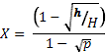
The RSWM is accessed in NetMap in the ‘Riparian Management Module’. Figure 2 showing the RSWM graphical user interface (GUI), that includes numbers in red, e.g. (1) that refer to numbers in this help document.
 Figure 2. RSWM Graphical User Interface. User inputs include (1) one or more stand tables, (2) average stand width for each stand, (3) average valley side slope for each stand, (4) thin and tip data (YYYY: XX), (5) average reach width, (6) the piece diameters that will be calculated by RSWM, (7) bank erosion rate = 0, (8) taper equation to be used in calculations of piece sizes and volume, (9) the tree fall direction type, (10) selections for tipping thinned trees, and (11) the decay rate for wood accumulation. Inputs, choices, and outputs are described below.
Steps include:
(1) Select a column in the reach table and click on Add Stand. Stands can be removed from the reach table by selecting them and clicking Remove Stand. Stand tables should be in comma delimited text format (.csv, .stb) with the following columns:
Stand ID: integer
Year: 4 digit integer
Species: 2+ characters
Diam Class: dbh in inches, integer
Live TPA: live trees per acre
Live Ht: live tree height in feet
ModelMort TPA: dead trees per acre for modeled tree mortality (e.g., forest growth models, FVS, ORGANON, Zelig, etc.)
ModelMort Ht: dead tree height in feet for modeled tree mortality
DiseaseMort TPA: dead trees per acre that died due to disease
DiseaseMort Ht: dead tree height in feet for diseased trees
InsectMort TPA: dead trees per acre that died due to insects
InsectMort Ht: dead tree height in feet
FireMort TPA: trees per acre that are subject to masswasting
FireMort Ht: dead tree height in feet
WindthrowMort TPA: trees per acre subject to wind throw
WindthrowMort Ht: dead tree height in feet
Total_thin TPA: total number of thinned trees per acre
Total_thin Ht: thinned tree height in feet
User_AquWood TPA: number of trees per acre tipped into stream
User_AquWood Ht: tipped tree height in feet
Example stand file:
Stand ID,Year,Species,Diam Class,Live TPA,Live Ht,ModelMort TPA,ModelMort Ht,DiseaseMort TPA,DiseaseMort Ht,InsectMort TPA,InsectMort Ht,FireMort TPA,FireMort Ht,WindthrowMort TPA,WindthrowMort Ht, Total_thin TPA, Total_thin Ht, User_AquWood TPA, User_AquWood Ht
2093048,1995,DF,46,2,31,1.1,31,0,0,0,0,0,0,0,0,0,0,0,0,0
2093048,1995,DF,54,1.1,31,0.4,38,0,0,0,0,0,0,0,0,0,0,0,0,0
2093048,2005,RA,58,4.1,40,0.1,100.3,0,0,0,0,0,0,0,0,0,0,0,0,0
2093048,2015,RA,28,4,50,0.1,100.4,0,0,0,0,0,0,0,0,0,0,0,0,0…
Column headings in italics must be spelled exactly as shown and headings must be all on one line. We recommend that all stands are stored in the same data directory as the data directory path is used to store result files. An example stand file follows:
When each stand table is read in, values are converted to metric for calculating wood recruitment using the conversions in Table 1.
(2) The average stand width must be entered in meters for each stand in the stand column in the table or by selecting the stand column and using the slider on the right side of the table.
(3) The average valley side slope must be entered in percent slope gradient for each stand or can be entered by selecting the stand column and using the slider.
(4) Tree tipping information is entered for each stand as appropriate using the format YYYY:XX where YYYY = a four digit year and XX is the percent or number of trees tipped from the thin. The thin information must be in columns in the stand table (see above).
(5) The average reach width must be entered in meters. This value can be calculated for all reaches in NetMap using the ‘Fluvial Morphology’ Module’. For a particular reach the value can be obtained using NetMap ‘Segment Attribute Information Tool’ in the ‘Basic Tool Module’.
(6) The diameter of output piece sizes can be entered in the box using the Add and Remove commands provided. The number of pieces of wood will be calculated using the range of these sizes. For example, if 0.1 m is entered, the number of pieces 0.1 m and above will be calculated. If values 0.1, 0.2, 0.5 m are entered, the number of pieces will be calculated for size ranges 0.1 to less than 0.2, 0.2 to less than 0.5 and all pieces greater than 0.5 m. The values default to 0.1, 0.35, and 0.6 m as these reflect the most common minimum diameter criteria for large woody debris (LWD) as determined by the National Marine Fisheries Service, US Forest Service, Bureau of Land Management, Washington Forest Practices Board, and Oregon Watershed Enhancement Board (Fox and Bolton, 2007).
(7) The bank erosion rate is set to zero on both sides of the reach (cannot be adjusted, because of issues with long term steady state channel width).
(8) A taper equation must be selected for conifer and hardwoods. Equations are used to calculate the tree diameter and the volume of pieces. Equation choices are from published papers by Kozak (1988), Waddell et al. (1987) and Hibbs et al. (2007). If the tree species is not recognized as a conifer or hardwood, calculations for it will default to the conifer equation selected.
(9) Tree fall direction can be calculated according to a) the directional bias calculated by Sobota et al. (2006) as described above or b) if slope is less than or equal to 40%, tree fall direction will be random and for slopes greater than 40% tree direction will be calculated according to Sobota et al. (2006).
(10) Thinned trees can be tipped into the stream by percent of thin (and number of thinned trees per acre). DBH (cm) ranges can be selected using the expressions indicated.
(11) The percent decay rate chosen for conifers, hardwoods, or default affects the amount of wood that accumulates in the stream.
Users can save a reach file containing the configuration of a model run for re-use, to facilitate sensitivity analysis, and to maintain a record of runs. Each reach can contain up to 6 stands; 3 stands on each bank. The reach file is comma delimited and the line format follows:
path/standfilename1
standID1
average stand width1
average valley side slope1
bank erosion rate
biomass calculation type
Lines ending in 1 can contain up to 6 values corresponding to different stands and stand information; places without stand information will contain 0s. The RSWM GUI allows users to open and save reach files. An example of a reach file with 5 stands follows:
Example Reach File
C:/Projects/WoodModel/504373thin70.csv,C:/Projects/WoodModel/504373NOthin.csv,C:/Projects/WoodModel/2093048.csv,---, C:/Projects/WoodModel/2093048.csv,C:/Projects/WoodModel/504373NOthin.csv,0
504373thin70,504373NOthin,2093048,---, 2093048, 504373NOthin,0
40,20,10,0,10,40
45,35,10,---,10,20,0
0.005
Cone
To calculate wood recruitment, click (12) Calculate; calculations will take several seconds and a pop-up message will inform you when they are complete (Figure 3).
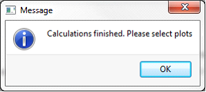 Figure 3. Calculations finished.
For each model run, RSWM generates an output file that is named OutTotalxxx.csv where xxx is a randomly chosen 3 digit number so that the file is not overwritten. Output files are saved to the folder that contains the stand tables. Users can generate their own custom plots from this file or use plots and plot files generated by RSWM.
After RSWM calculations are complete, the user can select one plot at a time to show the live or dead stand density from each input stand table in the drop down list (13), the numbers of pieces of wood per 100 m reach (14), or the volume of wood in cubic meters per 100 m reach (15).
(16) Users can chose to plot the number of pieces or volume of wood by distance to stream for selected piece sizes and by a selected year; by year for each piece size, by cumulative source distance by year, and wood accumulation over time (Figure 4). The user can save a plot to a .pdf or a .png file or build custom plots from the output file. When a plot is drawn, RSWM writes a text file containing the information in the plot. Stand density files are called either TPHLivexxx.txt or TPHDeadxxx.txt, where xxx is the stand ID: e.g., TPHDead504373thin70.txt. Files for distance to reach plots are called NPbyD2Syyyy.csv where yyyy is the 4 digit year, e.g., NPbyD2S1995.csv is the number of pieces by the distance to the stream for 1995. Files for the pieces size by time plot are called PieceSizeByTime.csv. OutTotalxxx.csv is the complete record of model calculations for each run; xxx is a random number so that this file is not overwritten. RSWM also writes to reach.txt with the details of the run and this is overwritten for each model run.
NOTES: Plot files will be overwritten each time the RSWM is calculated. RSWM Output and Plot files are written to the folder containing stand tables.
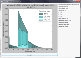 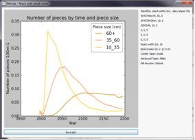 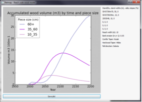 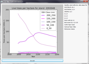 Figure 4. Example plots from RSWM.
(17) Click on Help to show this document or find the file at:
yourdrive\work\NetMap\manuals\RSWM_help.pdf.
(18) Click on Close to close all RSWM GUI and plot windows and return to NetMap.
Technical Background: Protecting riparian sources of wood for streams is becoming a major component of forestry policy in western states (Bisson et al. 1987, Bilby and Bisson 2004). Examples include establishing riparian protection zones for wood recruitment (Young 2000), mandating in-stream wood abundance standards or targets (NMFS 1996), monitoring abundance of wood in streams (Schuett-Hames et al. 1999) and implementing in-stream wood restoration programs (Cedarholm et al. 1997). The processes of forest mortality, bank erosion, streamside landsliding, debris flows and wildfires govern the supply of wood to streams (e.g., Murphy and Koski 1989, Benda and Sias 2003). The spatial distribution of different wood recruitment processes within a watershed or across landscapes varies substantially because of the diversity in forest composition and age, topography, stream size, climate and the history of natural and human disturbances (e.g., floods, fires, logging).
Spatial and temporal variability in wood recruitment processes can complicate the management and regulation of in-stream wood in both headwater channels (non-fish bearing) and larger fish bearing streams. For example, the width of riparian buffers to protect wood recruitment to streams may vary depending on whether forest mortality, bank erosion, or mass wasting is the dominant recruitment agent. If wood recruitment from channel migration or streamside landsliding is important, protection measures may extend up hillslopes beyond the streamside riparian forest (Reeves et al. 2003). Riparian forests could be managed for specific ecological objectives such as thinning dense young stands to increase the number of large trees (Beechie et al. 2000) or altering conifer-hardwood composition, strategies that require information on tree species and forest growth and mortality (Liquori 2006). Thus, an understanding of riparian processes that govern wood recruitment to streams can enhance protection strategies for riparian forests across physically diverse watersheds (Martin and Benda 2001).
There are a variety of modeling tools available for predicting wood recruitment to streams including RAIS (Welty et al. 2002), Streamwood (Meleason et al. 2003) and wood budgeting technology that addresses a range of recruitment processes including mortality, bank erosion, post fire toppling, landsliding and debris flow (Benda and Sias 2003, Benda et al. 2004).
NetMap contains tools for considering wood recruitment to streams including by mortality, bank erosion and debris flows. The reach scale wood recruitment model (RSWM) described in this manual addresses wood recruitment by forest mortality and bank erosion and is consistent with earlier models (Welty et al. 2002 and Meleason et al. 2003) except that it includes the process of bank erosion (e.g., Benda and Sias 2003).
|