| < Previous page | Next page > |
Probability of Salt Marsh and Mud flatsLayers representing the probability of saltmarsh (PSM) and probability of mudflats (PMF)
Layer Names: PSM_estuars, PSM_inund, PMF_estuars, PMF_inund
Layer Descriptions: PSM_estuars, PSM_inundsd, PMF_estuars, PMF_inund layers each contain the probability that a certain cell represents saltmarsh and mudflat, respectively. PSM_estuars and PSM_inund represent the probability of salt marsh habitat for the spatial extent of estuaries and the inundation layer (-100 to + 30 ft) respectively. Similarly, PMF_estuars and PMF_inund represent the probability of mudflat for the spatial extent of estuaries and the inundation layer. PSM_estuars and PMF_estuars are the complement of each other; similarly, PSM_inund and PMF_inund are the complement of the other.
Data Type: ESRI grid
Units: Probability
Description: Layers representing the probability of saltmarsh (PSM) and probability of mudflats (PMF) can be derived from the estuarine habitat model which was developed for the Puget Sound using the inundation layer and training points in Google Earth. The Puget Sound has many estuarine areas (Figure 1), several of these are drained and the land reclaimed for agriculture and other uses.
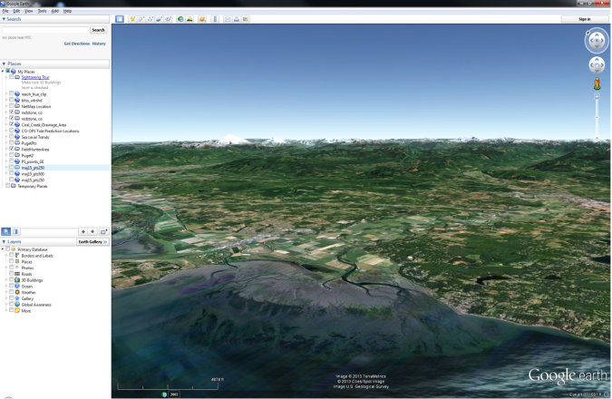 Figure 1 Skagit River, Puget Sound
The 100 training points identified areas of saltmarsh (red) and mudflat (blue) (Figure 2). Salt marshes stabilize estuarine sediment with vegetation – sedges, fescues, asters; habitat; it is likely that they experience less than 50% annual inundation. Mudflats or intertidal zone is frequently inundated, provides habitat and foraging for shorebirds and raccoons.
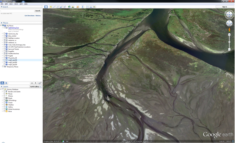 Figure 2 Areas of saltmarsh (red) and mudflat (blue) used to get training points for the estuarine habitat model.
The training points were plotted against inundation values for the points to determine whether this would give enough information to derive a model (Figure 3). Initially we tried 7 categories including lower mudflat, mudflat, upper mudflat, lower saltmarsh, salt marsh, upper salt marsh, and non-tidal. The differences between upper and lower were not easily distinguished in the training points so we dropped this distinction and focused on the main classes: mudflat and saltmarsh. Most of the non-tidal points were at 0 % inundation as expected. The two non-tidal points in inundated areas were identified as borderline points close to channels and the coarse resolution of the inundation grid resulted in these being misclassified. Non-tidal points were dropped from model development.
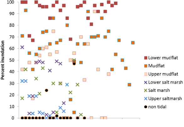 Figure 3 Percent inundation versus habitat classifications for mudflat, saltmarsh and non-tidal.
The slope of the estuary may also determine the habitat class (Dyer et al 2000) so we extracted percent slope values calculated from a 30 ft. resolution DEM http://www.ocean.washington.edu/data/pugetsound/psdem2005.html. Accessed 2013. (Finlayson, 2006). The plot of slope values versus inundation for the training points showed that there was no relationship between slope and inundation for the selected area (Figure 4) and slope was dropped from the model.
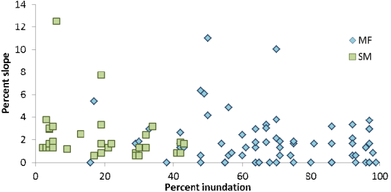 Figure 4 Percent slope v. percent inundation
Using only the training points and percent inundation (%Inund) we developed a logistic regression model to determine the probability of saltmarsh (PSM) or mudflat. The model is given by:
The model determines that above 50% inundation is generally mudflat but below 50% inundation may be a mix of saltmarsh and mudflats (Figure 5).
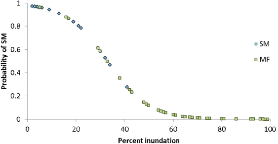 Figure 5 Probability of Salt Marsh, colored by model training points
The model was validated using 126 points that were randomly generated in the estuarine areas of the Puget Sound. The higher prevalence of mudflat points reflects the ubiquity of mudflats compared to areas of saltmarsh. From the error matrix (Table 1), we calculated the kappa statistic to be 0.57 which is generally characterized to be moderate to good agreement between validation points and the model (Landis and Koch, 1977).
Table 1. Error matrix comparing values of the validation points to the estuarine habitat model points.
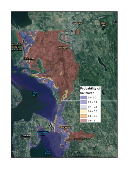  Figure 6. Comparison of the probability of saltmarsh (left) with wetland map derived from historic sources on the Skagit and Stillaguamish deltas (right; Collins, 2008).
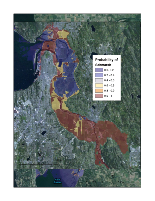 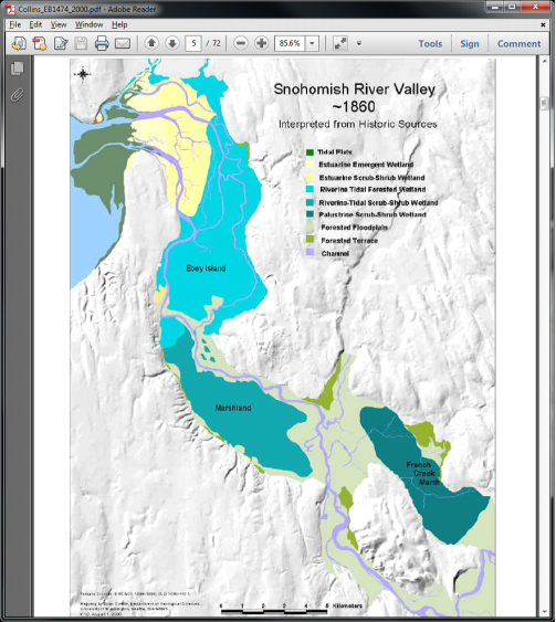 Figure 7. Comparison of the probability of saltmarsh (left) with wetland map in the Snohomish Valley (right; Collins, 2008)The probability of saltmarsh (PSM) layer represents current agricultural areas in the Skagit, Stillaguamish, and Snohomish estuaries as having a high probability of being saltmarsh (Figures 6 and 7). Historic sources reveal that these areas, which are now diked and drained, may have originally been one of several different types of wetland, either estuarine, riverine, or palustrine. It is not as easy to determine the type of vegetation in each wetland. In the Skagit and Stillaguamish, areas that are likely to be mudflat (i.e. with low probability for saltmarsh), tend to be in areas delineated as estuarine wetlands. Areas with a high probability of saltmarsh were mapped historically as riverine or palustrine tidal scrub-shrub, riverine or palustrine tidal forested wetlands or forested floodplain. The mouth of the Snohomish, which was historically tidal flats, is mapped as expected with a high probability of mudflats (Figure 7). Further inland of the mouth of the Snohomish, an area mapped as likely saltmarsh, was historically estuarine emergent or scrub-shrub wetland.
In Figure 6, the orange oval indicates an error in the DEM which is reflected in the sharp north-south line in PSM on the estuary where there is no sudden drop in the landscape.
The significance of this model lies in its facility to quickly and easily map habitat types using only topographic data. Further runs of the inundation model could be used to determine the impacts of climate change and sea level rise on habitat in estuaries. Improvements may be made in the future using remotely sensed imagery. See also help for the inundation layer.
References
Dyer KR, Christie MC, Wright ER, 2000. The classification of mudflats. Continental Shelf Research 20: 1039-1060.
Finlayson DP, 2005 Combined bathymetry and topography of the Puget Lowland, Washington State. University of Washington, (http://www.ocean.washington.edu/data/pugetsound/)
Finlayson, DP, 2006. The geomorphology of Puget Sound beaches. Puget Sound Nearshore Partnership Report No. 2006-02. Published by Washington Sea Grant Program, University of Washington, Seattle, Washington. Available at http://pugetsoundnearshore.org. Accessed 2013.
Landis, JR, Koch GG, 1977. "The measurement of observer agreement for categorical data". Biometrics 33 (1): 159–174. doi:10.2307/2529310. JSTOR 2529310. PMID 843571.
|