| < Previous page | Next page > |
Model #2 Partial BBN - Habitat Intrinsic PotentialModel #2, Partial BBN – Habitat Intrinsic Potential
To simplify the full BBN model of Peterson et al. (2008), NetMap includes a partial BBN to estimate the “intrinsic potential” of westslope cutthroat trout habitat. The model includes the parameters of channel physical attributes of gradient, width and temperature. This version of the BBN works the same as described above for the full version. The Field attribute name is PWCT_IP.
User inputs are a shapefile of selected stream reaches with reach gradient (m/m), stream temperature (°C), and stream width (Figure 4). Users can select a stream temperature field if one is available in their reach shapefile (NetMap does not provide this as of 2011) or they can select a constant value from the drop down box. Users can select bankfull width or wetted width as input. If bankfull width is chosen, NetMap will convert it to wetted width using the default linear regression or using other intercept and coefficient values provided by the user. The default linear regression equation (R2 = 0.61; p = 2.20E-16) which converts bankfull to wetted width was developed for stream reaches surveyed by the Kalispel Tribe Initiative, Pend Oreille County, WA.
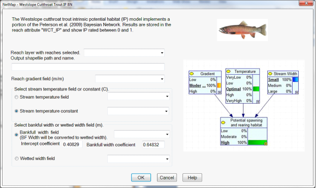 Figure 4. User interface for the NetMap westslope cutthroat trout intrinsic potential Bayesian network model (after Peterson et al. 2008).
The WCT_IP BBN results in probabilities being assigned to each state (low/poor, moderate/suitable, high/optimal) for the node. There are six combinations of node state probabilities and these are assigned to one value from the list: 0, 0.2, 0.4, 0.6, 0.8, or 1.0 according to the habitat quality. This list value is written to the stream reach for which it is calculated in the attribute PWCT-IP (Table 2). The reach shapefile is mapped automatically using this attribute (Figure 5).
Table 2. Node state probabilities assigned to PWCT-IP.
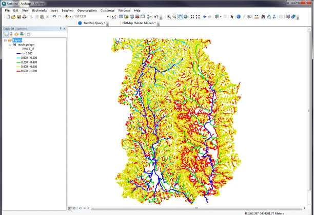 Figure 5. An example of mapped PWCT_IP. Red color code indicates high intrinsic potential for West slope cutthroat trout.
Technical Background: Bayesian belief networks (BBNs) are models, based on Bayesian probability theory, for reasoning about uncertainty (Jensen et al. 1996). When there is no past history to help solve a complex problem, a BBN can be defined to find a solution. BBNs can help make explicit the results of a series of dependencies and causal connections to calculate a probability.
A BBN is a directed graph of nodes and Fields with a set of conditional probability tables. The BBN graph consists of nodes that represent model variables and Fields that connect the nodes; each Field has a direction showing how the “from” or “parent” node influences the “to” or “child” node. For example, in Figure 4, gradient, temperature, and stream width are all parent nodes; potential spawning and rearing habitat is the child node and network result; all child nodes have an associated conditional probability table. Conditional probability tables contain probabilities that quantify the node response to parent nodes and the uncertainty in that response. For example, states for the gradient node are low, moderate, and high. The combination of probabilities from each parent node is used to calculate the state of the child node.
Many things that you would like to know about Bayesian networks, you can find, in very readable format, here: http://www.eecs.qmul.ac.uk/~norman/BBNs/BBNs.htm.
All Bayesian networks in NetMap are calculated using Smilenet which is freeware from the Decision Systems Laboratory, University of Pittsburgh (http://dsl.sis.pitt.edu) within a Visual Basic and FieldGIS framework. If you are interested in developing a BBN, you can use the Genie shareware, also from U. Pittsburgh.
|