Gullying

Gully Erosion

Parameter Description: The susceptibility of hillslopes to gully erosion.

Important Notice: This erosion model is not calibrated for any particular landscape. Although the model employs universal topographic indicators of gully erosion potential increased accuracy and resolution can be obtained when the model is calibrated using local data (georeferenced locations of landslides or gullies). A calibration tool is planned for NetMap in later 2014. Also see Warning about using Slope Stability Models.

Data Type: Grid; Line (stream layer)

Field Name: Gully_dataset name; Common Name: Gully Erosion Grid

Field Name: Gully_LOC; Common Name: Gully Erosion - Segment (summed to reach from drainage wings)

Field Name: Gully_CUM; Common Name: Gully Erosion - Summed Downstream

Units: Relative Index

NetMap Module/Tool: Erosion Processes/Gullying

Model Description:

NetMap’s gully model employs the Compound Topographic Index (CTI) as a predictor of ephemeral gully potential (Parker et al. 2010). CTI is calculated for each grid cell in NetMap's Digital Hydroscape. CTI is defined as:

CTI = A * S * PLANC

where A is the upstream drainage area (L²), e.g., the number of pixels draining to any point on the landscape, S is the local slope (L/L), which combined is a proxy for runoff discharge, and PLANC is the planform curvature (1/L), a measure of hillslope curvature (negative for ridges and positive for swales) (Zevenbergen and Thorne 1987).

A user first provides an area threshold to limit the gully erosion prediction into the fluvial network (1 km² is the default). Running the two creates three outputs: 1) hillslope prediction (grid), which can include channel cells, 2) gully potential reported to reaches and 3) gully in reaches (gully values summed via drainage wings), summed (aggregated) downstream.

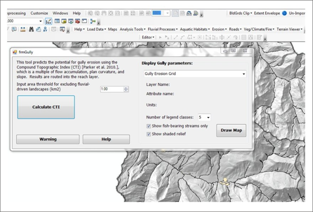Figure 1. The gully tool interface. A user inputs an area threshold and then proceeds to calculate gully erosion potential.

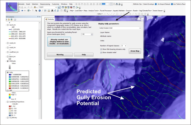Figure 2. An example of the gully erosion potential grid.

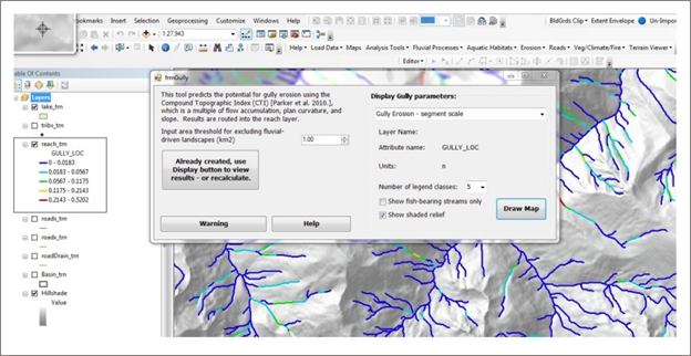Figure 3. An example of the gully erosion potential in reaches. The reach scale prediction of gully erosion represents the drainage wing sum of gully erosion potential. Segment scale values are summed downstream providing a running sum (downstream) of total gully erosion potential, useful for considering tributary scale variation in hillslope gully erosion potential. These parameters could be considered in the context of fire probability and fire severity.

Background:

Taken from Parker et al. (2010)

Zevenbergen (1989) describes five factors as influencing ephemeral gully formation including:

1.Overland flow discharge and duration, without which ephemeral gullies could not exist;

2.Slope and flow depth, which determine the magnitude of the flow’s downslope component of

weight and, therefore, the boundary shear stress exerted by the flowing water on the soil;

3.Planform curvature, which determines the local flow convergence and, therefore, the

concentration of stress along a flow path or swale;

4.Soil characteristics, which affect both overland flow rates (through controlling infiltration

capacity) and determine the erodibility of the soil;

5.Vegetation characteristics, which affect overland flow rates through interception and flow

resistance and provide cover for the soil, reducing its susceptibility to erosion.

Recent work on the controlling influences of gully development has identified enlargement of

pipes through subsurface flow as a critically important soil erosion process which can be

responsible for exceptionally high soil losses (Faulkner, 2006). While this study is aware of this

process it is beyond the scope of the technique developed here which aims to focus solely on

topographic controls of overland flow important in influencing ephemeral gully development.

In terms of topographic influence Thorne et al. (1984: 2) identified that “the formation of an

ephemeral gully depends on the generation of concentrated surface runoff of sufficient

magnitude and duration to initiate and maintain erosion, leading to channelisation”. From this,

the first three of the above factors listed by Zevenbergen: discharge, slope and planform

curvature, are key topographic controls in the formation process.

The importance of these three factors can be theoretically considered using stream power, a

parameter commonly used to represent flow intensity and predict sediment carrying capacity

(Bagnold, 1966; Yang, 1977). The concentration of surface runoff described by Thorne et al.

(1984) can be physically represented by specific stream power, which is a function of discharge,

slope and width. Drainage area is often used in geomorphic analysis as a surrogate for discharge

and, consequently, drainage area multiplied by slope gives a parameter acting as a proxy for total

stream power. This line of argument justifies the inclusion of both slope and drainage area (as an

acceptable surrogate for discharge) in a technique responsible for predicting the formation of

ephemeral gullies.

The third topographic factor, planform curvature, or convergence, contributes to ephemeral gully

formation in multiple ways. Firstly, without convergence runoff volume and discharge are

linearly proportional to slope length, while with convergence these values are related to slope

length to a power greater than unity (Zevenbergen, 1989). Secondly, at any point along a swale

in the downstream direction the degree of planform curvature determines local flow geometry,

including the degree of flow concentration. This means that the level of convergence in the land

surface is important in controlling the initial flow path geometry, and therefore, the initial

channel location. In other terms, whilst the product of slope and discharge may adequately

represent total stream power, planform curvature is necessary to represent the degree of

concentration of this stream power and so enables it to become a representation of specific

stream power, the key component of Bagnold’s sediment transport theory.

Zevenbergen and Thorne (1987) developed a methodology for calculating slope, aspect,

planform curvature and upstream drainage area for each point within an elevation grid matrix.

2nd Joint Federal Interagency Conference, Las Vegas, NV, June 27 - July 1, 2010Thorne et al.

(1986) used these parameters to calculate a Compound Topographic Index (CTI)

for each grid cell within that matrix, which is used to identify potential locations for ephemeral

gullies based on land topography. The CTI is defined by:

CTI = A · S · PLANC (1)

where: A = upstream drainage area (L2) and provides a surrogate for runoff discharge since the

two are generally strongly positively correlated; S = local slope (L/L), which together with

upstream area provides an indication of the stream power per unit downstream distance of the

runoff; and PLANC = planform curvature (1/L), a measure of the landscape convergence

(negative for spurs and positive for swales) indicating the degree of concentration of the runoff

and so allowing the CTI (L) to represent specific streampower (streampower per unit bed area).

As a result, the CTI represents the major parameters controlling the pattern and intensity of

concentrated surface runoff in the field.

This study aims to take the work carried out by Zevenbergen and Thorne during the 1980s

forward, utilising the contemporary advancements of Geographical Information Science (GIS) to

automate the derivation of the CTI parameter from Digital Elevation Models (DEMs). This paper

describes the development and initial testing of the GIS based CTI process as well as

considerations for the impact that DEM resolution and source can have over the process’s

results.

Made with help of Dr.Explain