| < Previous page | Next page > |
|
Drainage Wings: River Network – Terrestrial Coupling
Just like real landscapes, terrestrial landforms are connected to river networks within a Digital Hydroscape by grid cell referencing. Downslope–upslope transfer of information, and vice-versa, addresses processes such as sediment moving from hillsides to rivers or animals transferring nutrients from streams and riparian zones to mid slope forests. Each river cell is linked to adjacent or nearby floodplain, terrace or valley cells, allowing riparian environments to be coupled to specific reaches of channel. For instance, riparian forests drive recruitment rates of in-stream wood and are directly related to formation of fish habitat (e.g., pools, cover), a relationship that ties spatial locations of valley floors and channels together.
Local drainage contributing areas, called "drainage wings", are delineated on both sides of individual channel segments in a Digital Hydroscape (Figures 1 and 2); i.e., channels discretized between 50m and 200m create drainage wings of tenths of a square kilometer in area. Terrestrial attributes at the drainage wing scale, such as lengths of roads and pipelines, vegetation type and age, erosion risk, etc., are summarized at that scale and are used to characterize those environments (Figure 1). Terrestrial information is transferred to channel segments as well, allowing hillslope information, including those representing resource uses and infrastructure (drilling pads, roads, forest harvest etc.), to be directly related to in-channel environments, including aquatic habitats. Data at the scale of drainage wings and individual channel segments are aggregated downstream or upstream (often referred to as “routed” in a GIS), revealing patterns of terrestrial (or in-channel) attributes at any spatial scale defined by the river network.
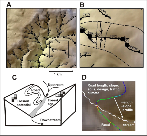 Figure 1. The Digital Hydroscape includes (A) a routed analytic river with confluences, including with attributes (Table 1). (B) Each segment has a right-left differentiated local contributing area or Drainage Wing (tenths of a square kilometer at segment length of 100m). (C) Information contained within Drainage Wings, such as erosion potential, fire risk and road length, is transferred to stream segments. Information can also be aggregated downstream, revealing patterns of channel and hillslope characteristics at any spatial scale defined by the channel network. Drainage Wings support spatial analyses including identifying overlaps between terrestrial and riverine environments, including human related stressors (such as erosion, wildfire, roads etc.). (D) Roads (pipelines and power transmission lines) are broken at pixel borders to link road segments to pixel scale information on factors such as landslide potential; road pixel segments can also be re-aggregated to predict factors such as road drainage diversion potential.
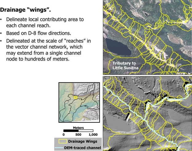 Figure 2. Drainage wings are on the order of 0.1 km2 in area, but variable depending on synthetic stream reaches (typically between 50 and 200 m in length) and topography. The small stream segments and corresponding drainage wings allow for fine scale discretization of the terrestrial landscape to map in detail habitats and land use and habitat interactions.
 Figure 3. The shapes and sizes of drainage wings vary based on stream segment length and topography (and relief). This image shows a watershed divided up into drainage wings.
Roads, railroads, energy pipelines and power transmission lines are discretized, breaking the data that represents them at pixel cell borders so that small sections of roads and pipelines (e.g., grid cell size) can be evaluated at the corresponding grid cell scale of the hillslope and analytic river. These linear features can be associated with similarly scaled indices of other landscape attributes such as erosion potential (Figures 1 and 2). Roads or pipelines that cross hillside grid cells are linked to channel cells via surface flow paths, thus providing a means to evaluate how roads and pipelines might affect fish habitats or water quality. Small road sections can be reaggregated to any scale, including that of Drainage Wings, such as road drainage (or pipeline) diversion potential. Data at these multiple scales can be used to link hillslope erosion (surface, landslides, debris flows) to specific roads and pipelines and then to individual stream segments.
The spatial referencing of roads and pipelines, in combination with river routing of information in a Digital Hydroscape, can lead to innovative solutions to environmental needs, such as toxic spill response. For example, any location in a river network, such as municipal water intakes, can be characterized by a series of transport times and dilution rates from an upstream population of pipeline-stream crossings, or other energy development infrastructure in close proximity to water courses related to energy development.
NetMap’s data structure allows the cumulative distribution of any watershed or resource use attribute to be calculated on the fly at any scale. This structure allows terrestrial information (such as erosion potential) or road and pipeline density (km km-2) to be evaluated in terms of exceedence frequency or probability. Thus, a planner can quickly assess whether Drainage Wing’s with the highest 10% of erosion potential (due to roads) overlap with the top 10% of the most sensitive river channels. Identifying such locations could be used to prioritize areas where remedial efforts, such as road maintenance, would have the greatest benefit to freshwater ecosystems.
The geospatial data structure of a desktop watershed analysis should be customizable to individual watersheds and landscapes. Analytic river networks can be expanded or contracted, and segment lengths and Drainage Wings can be decreased or increased in size, to meet the needs of particular applications. Thus the data structure (such as the analytic river) is not fixed in space and time, but rather it is dynamic, ensuring that analyses remain accurate and relevant. In addition, knowledge generated within an analytic stream layer (NetMap) can be transferred to other agency and private sector stream layers and vice versa.
Use of drainage wings, with information transferred to stream segments, offers greater insights into the spatial variability of watershed attributes. For example, road density (km/km2 or mi/mi2) is typically calculated at the scale of watersheds. Density values are often in the range of 1 to 5. However, when road density is mapped at the scale of individual drainage wings, density values can range from zero to a couple of hundred (Figure 3). Thus drainage wings can be used to create maps of variation in roads, and thus potential road impacts, at a high resolution. See also the Road Density Tool.
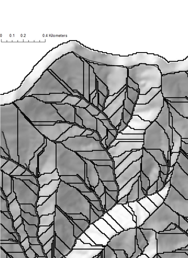 Figure 4. Calculating road density at the stream segment scale (e.g., drainage wing scale) produces a much higher resolution of variations in road density. For example, road density in the Clearwater Basin (MT) that is calculated at the scale of HUC 6th field subbasins ranged between 0.5 km/km2 and 4 km/km2 (top). In contrast road density measured at the stream segment scale ranged between zero and 100 km/km2.
|