Road Surface Erosion & Delivery
Model Descriptions:
The WEPP road surface erosion model and the GRAIP-Lite mode is used within NetMap; see tools here and here.
WEPP example below.
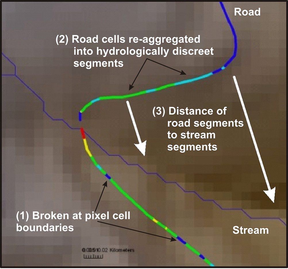
Figure 1. In NetMap, road layers (lines) that may be kilometers long are broken at pixel cell boundaries (1). They are then re-aggregated into hydrologically discreet segments between topographic high and low (pour) points using NetMap's road drainage tool. These segments are used in the WEPP road surface erosion model. In addition, each road segment is linked (by distance and hillslope gradient) to the nearest downslope channel segment, called the “buffer” in WEPP, that influences the potential for road sediment to enter streams.
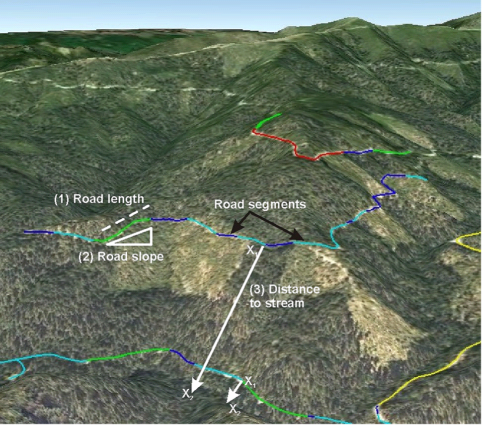
Figure 2. Important factors of road surface erosion include road segment length (1) that is hydrologically distinct (shown by the different color codes, the slope of the road (2), and the distance of individual road segments (drain or pour points) from individual stream segments (3). A simple index or proxy of road surface erosion (Road Erosion Index tool) uses these three parameters.
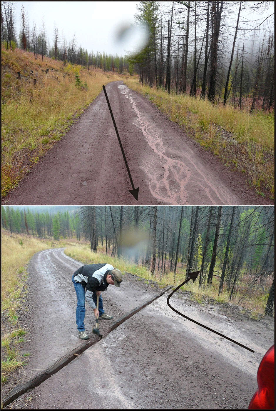
Figure 3. (Top) Long stretches of road can be hydrologically connected, via overland flow. In the Clearwater River basin that can lead to considerable surface erosion and the delivery of both fine sediments and other materials (nutrients) to streams. (Bottom) The use of cross drains (a form called ‘open tops’ in the photo) can be used to decrease the length of overland flow and thus decrease the amount of surface erosion and the volume of sediment and other materials reaching stream channels. Arrows illustrate the accumulation of flow and its disruption due to the cross drain, during conditions of light rain.
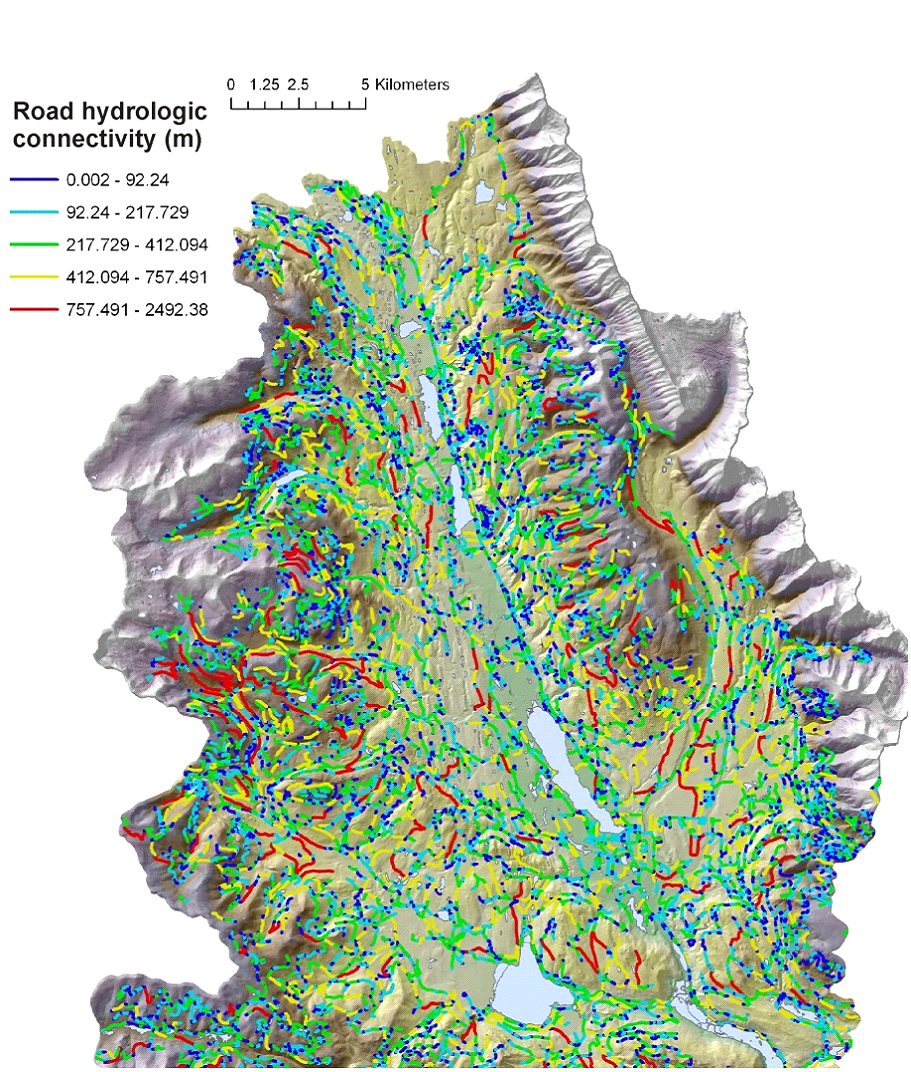
Figure 4. Predicted road hydrologic connectivity ranged between ten and 2500 meters (average 133 m). This parameter, during large storms or following fires when secondary drainage structures may be compromised, could be viewed as an index of ‘road drainage diversion potential’. The drainage diversion index could be used to identify locations where field crews could check on drainage efficacy during or after storms or following fires.
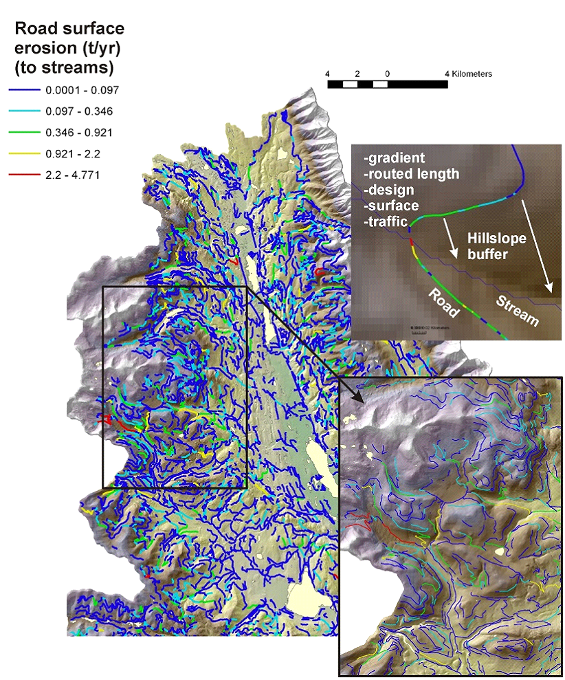
Figure 5. Road surface erosion (as delivered to streams) in the Clearwater basin ranged from very low (near zero) to a maximum of 4.7 tons/year. In the figure, individual road segments are color coded according to predicted annual sediment yield. Predicted sediment yields to streams are sensitive to the hillslope distance and gradient (e.g., buffer) from individual road segments to streams, as illustrated in the figure (upper right).
GRAIP Lite Model below:
The eight types of output are shown below in Figures 6 through 13.
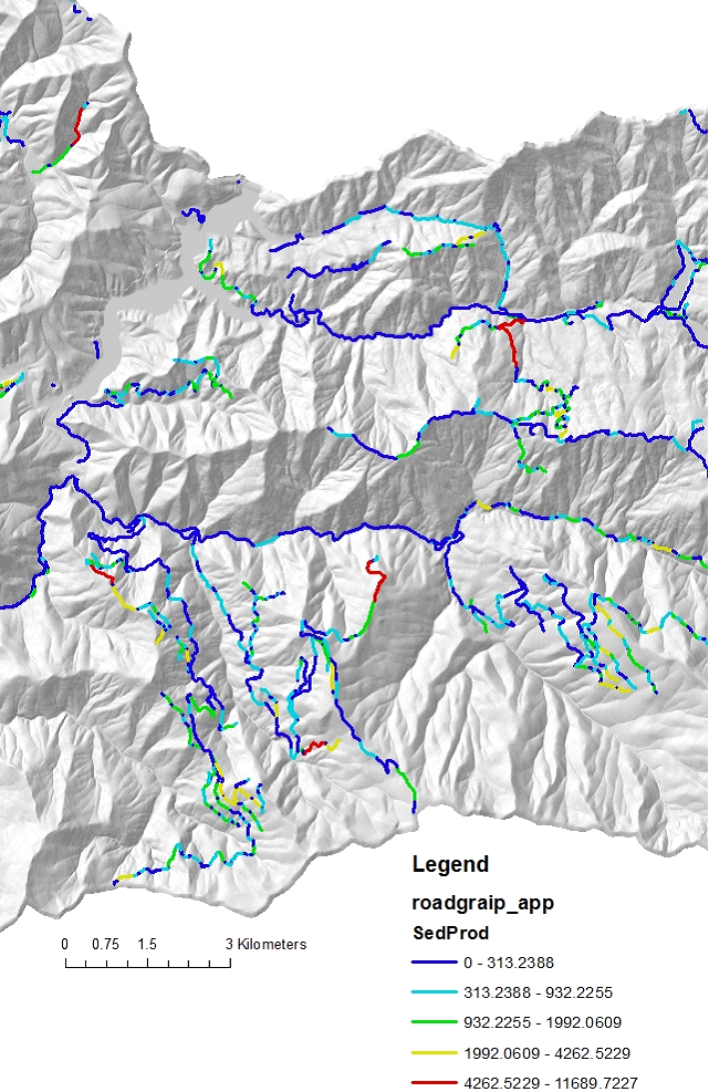
Figure 6. GRAIP road sediment production, kg/yr, (in the GRAIP road layer). Delivery to streams is not considered.
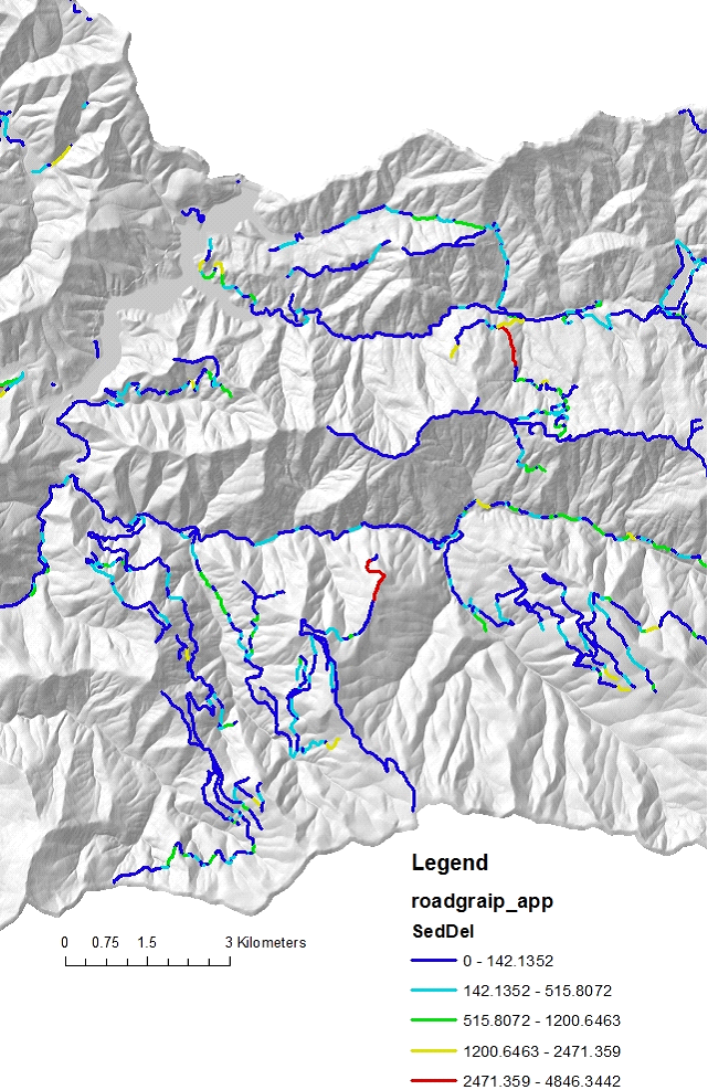
Figure 7. GRAIP road sediment production, kg/yr, delivered to streams (in the GRIAP road layer).
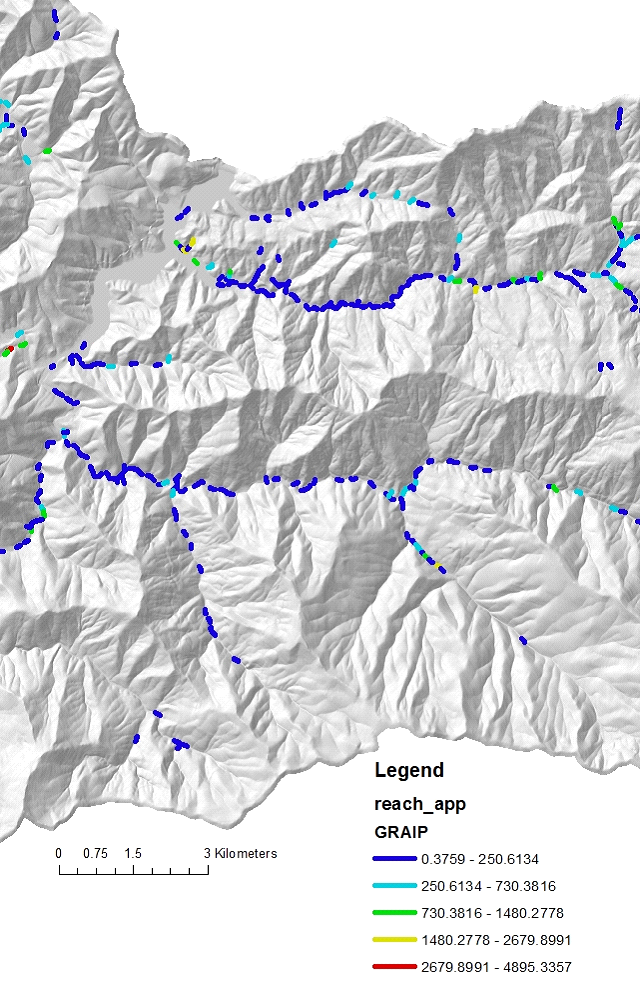
Figure 8. GRAIP road sediment production, kg/yr, delivered to streams (in the reach layer, per stream segment).
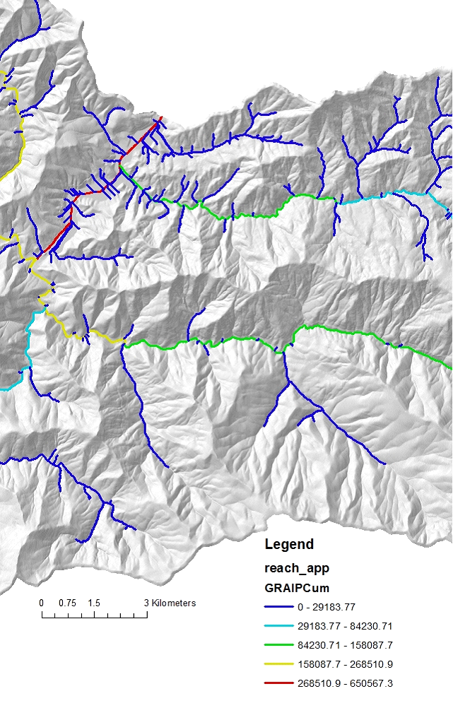
Figure 9. GRAIP road sediment production, kg/yr, delivered to streams and routed (area weighted) downstream (in the reach layer).
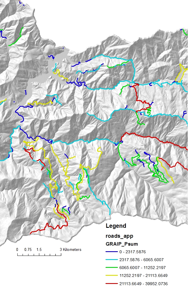
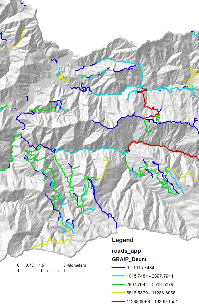
Figure 10. GRAIP road sediment production, summed in kg/yr, reported back to original road layer (referenced to unique road IDs).
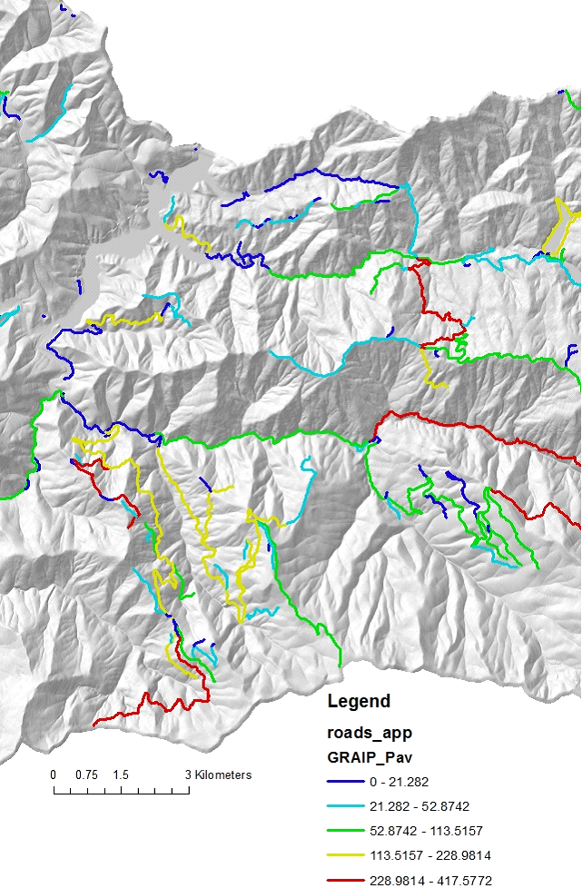
Figure 11. GRAIP road sediment delivery to streams, summed in kg/yr, reported back to original road layer (referenced to unique road IDs).
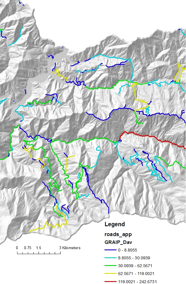
Figure 12. GRAIP road sediment production, length weighted in kg/yr/m, reported back to original road layer (referenced to unique road IDs).
Figure 13. GRAIP road sediment delivery to streams, length weighted in kg/yr/m, reported back to original road layer (referenced to unique road IDs).