| < Previous page | Next page > |
GRAIP-LiteGeomorphic Road Analysis and Inventory Package (GRAIP-Lite)
(Developed by the Forest Service Rocky Mountain Research Station [RMRS] and Utah State University). Charlie Luce, Thomas Black, Nathan Nelson.
Parameter Description: Predicted erosion (sediment production) from road surfaces and predicted sediment delivery in channels.
Data Type: Line (road layer, stream layer)
(1) Field Name: SedProd (RoadGRAIP layer); Common Name: GRAIP Sediment Production
(2) Field Name: SedDel (RoadGRAIP layer); Common Name: GRAIP Sediment Delivery (to channels)
(3) Field Name: GRAIP (Reach layer); Common Name: GRAIP Sediment Delivery to reaches
(4) Field Name: GRAIPCum (Reach layer); Common Name: GRAIP Sediment Delivery to reaches-summed
(5) Field Name: GRAIP_Psum (original road layer); Common Name: GRAIP Sediment Production – summed (reported back to road segment IDs)
(6) Field Name: GRAIP_Dsum (original road layer); Common Name: GRAIP Sediment Delivery-summed (reported back to road segment IDs)
(7) Field Name: GRAIP_Pav (original road layer); Common Name: GRAIP Sediment Production-per meter (length weighted, reported back to road segment IDs)
(8) Field Name: GRAIP_Dav (original road layer); Common Name: GRAIP Sediment Delivery-per meter (length weighted, reported back to road segment IDs)
Units: kg/yr
NetMap Module/Tool: Roads
Model Description:
The Geomorphic Roads Analysis and Inventory Package is designed to learn about the impacts of road systems on erosion and sediment delivery to streams. As the name implies it couples an inventory to analytical tools to build an approach to roads analysis that can be locally calibrated in a repeatable fashion with minimal effort. The full scope of GRAIP includes methods to inventory roads and analyze the inventory for surface erosion, gully risk, and landslide risk; methods to measure surface erosion from sample sites; and methods to estimate surface erosion where no inventory has been taken. From Charlie Luce and Thomas Black (2012), Appendix 1. Refer also: http://www.fs.fed.us/GRAIP/intro.shtml.
GRAIP-Lite is the GIS version of GRAIP and it was designed to quickly prioritize watersheds based on road-related sediment production and delivery. It requires a road layer embedded within a GIS. In NetMap, the road layer is integrated within a Digital Hydroscape. GRAIP-Lite requires calibration datasets to calculate road erosion and they are included in NetMap’s GRAIP interface. Users are encouraged to apply the full GRAIP technology to develop calibration datasets for their own landscapes.
Road sediment production is predicted by: E = B*R*S*V (1)
where E is road sediment production (kg/yr), B is the base road surface erosion rate, R is the elevation difference between the road segment end points, S is the road surface factor and V is the vegetation factor. V and therefore E are calculated separately for each combination of road surface type and road maintenance level. V = 1 - 0.86x where x is the fraction of the road where flow path vegetation is greater than 25%.
Field measured base erosion rates (kg/yr) exist for Oregon Coast Range, sandstones (79 kg/yr); Idaho Batholith, Granitics (33 kg/yr); Montana, Belt Series Meta sedimentary (7 kg/yr); and Eastern Oregon, Umatilla River, Basalt (1.5 kg/yr). The vegetation factor calibration data sets exist for Seeley, Montana; Siuslaw River, Oregon Coast Range; Umatilla River, Eastern Oregon; Idaho, Middle Fork Salmon; Idaho, Middle Fork Payette; and Idaho South Fork Salmon. A “master” vegetation calibration dataset that is the average of all of them is also included in NetMap’s GRAIP-lite interface.
A road layer (such as US Forest Service road lines, each with unique IDs) is broken into segments to mimic the spacing of drain points. NetMap’s Road Drainage tool is used to calculate road segment length scales (Figure 1).
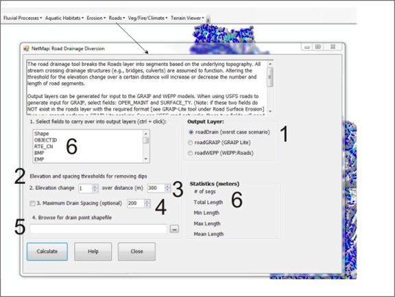 Figure 1.NetMap’s road drainage tool allows users to custom set the drain spacing along road segments to use with road surface erosion predictions (using GRAIP-Lite or WEPP) and for estimating worse case scenarios when secondary drainage structures are non functioning because of large storms or following wildfires. This tool assumes that all road-stream crossings function, with drainage going from roads to streams at those locations. (1) A user selects the output layer desired (GRAIP, WEPP or road drainage diversion). (2) An elevation change is selected (the change in elevation along the road necessary to define road drain or pour points. (3) A road length distance is selected over which the elevation change (2) is calculated over. (4) A maximum road spacing can be specified. (5) A user can import their own GPS road drainage location data points (in the form of an Arc point shape file). (6) The average, minimum and maximum road segment lengths that are generated are displayed. (6) Attributes in the original road layer (such as road ID) can be carried over into the delineated segments. See Table 1 below for a sensitivity analysis of how change in elevation (2) and distance (3) influences the predicted road segment length.
Table 1. A sensitivity analysis that shows how elevation change and distance (#2 and #3 in Figure 1) will affect the average and maximum length of road segments for use in GRAIP, WEPP and worst case drainage diversion.
Once road sediment production is calculated (E), the proportion that is delivered to streams is highly sensitive to the distance of the road to the stream. NetMap calculates the distance of each road segment to the corresponding stream segment that it drains into. Field studies during GRAIP analyses have indicated a significant reduction in sediment delivery with increasing distance of the road from the stream (Figure 2). The average of those curves is used in NetMap’s GRAIP tool to predict the fractional proportion of sediment delivery to streams from forested roads (Figure 3). The effect of distance to stream is significant: roads located less than 200 m from a stream are predicted to deliver greater than 40% of sediment to stream channels; roads located greater than 200 meters from streams are predicted to delivery approximately less than 5% of sediment.
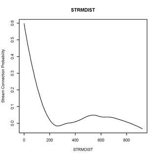 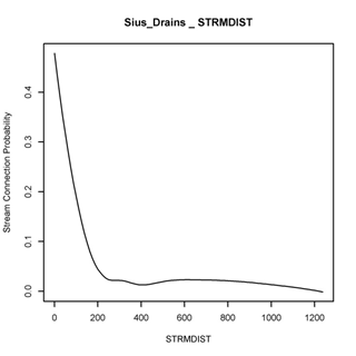 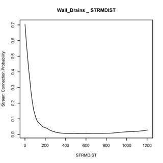 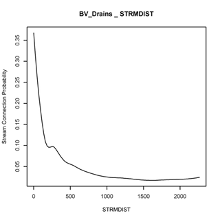 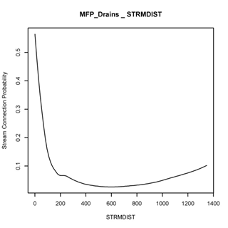 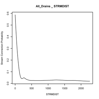 Figure 2. Fractional sediment delivery curves from five different landscapes based on GRAIP field studies.
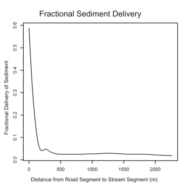 Figure 3. The average of fractional sediment delivery curves (All_Drains in Figure 2) is used in NetMap’s GRAIP tool; but note that NetMap contains an alternative model to predict road sediment delivery to streams (see below).
The GRAIP tool interface in NetMap allows a user to select a base erosion rate from a drop down list of available sites or to estimate a rate based on professional judgment (Figure 4). The vegetation factor source relationship is selected next, using either the master average or one of the empirical data sets. For this step, two attributes in the correct format in the road layer are necessary: 1) Road maintenance level and 2) Road surface type. Note that these attributes need to be in a specific format. For road maintenance level, the attribute field must start with a numerical values of 1 to 5 (i.e., 2 – high clearance vehicles). For road surface type, the attribute field must have the following categories (AC, AGG, NAT, IMP) which refers to paved, crushed rock, native and improved native. These attributes are standard in US Forest Service road layers. In other jurisdictions and with other road layers, these categories will need to be added, in the correct format, if GRAIP-LITE results are desired. A minimum road slope can also be indicated if a user knows that road line work is inaccurate in certain areas leading to spurious (high) road gradients (Figure 4).
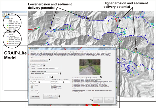 Figure 4. NetMap’s GRAIP interface. (1) A user must first define the length scale of the road segments to be used (e.g., distance between road drain points). This is done using NetMap’s Road Drainage Diversion tool (Figure 1). (2) A road erosion base rate is either selected from the drop down list of available empirical values or a rate is given (known or guessed). (3) A calibration data set is chosen from the drop down list of available empirical values. (4) A maximum road slope can be defined, if there is reason to believe that the GIS road layer is not sufficiently accurate (thus leading to spuriously high road gradients). (5) Ff the road maintenance and road surface types are in the correct (USFS) format, they are automatically carried over from the original road layer when the road GRAIP road layer is created; if another format is used, #5 and #6 allow a user to select them. Caution: at times, ArcMap will not carry over the road maintenance or road surface type fields into the new attribute table of the road GRAIP layer – if the tool indicates that one or more of those fields are missing, close ArcMap and reopen, to clear out the shapefile cache. You might have to do this more than once (an ArcMap limitation). (7) The GRAIP-Lite model is run. (8) A user selects from two different types of road sediment delivery to streams, either the GRAIP-Lite version (see above, Figure 3) or NetMap's conservation of mass sediment delivery model (see below). (9) The multiple types of model output is listed. (10) Technical Help is available (this document).
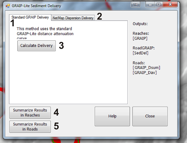 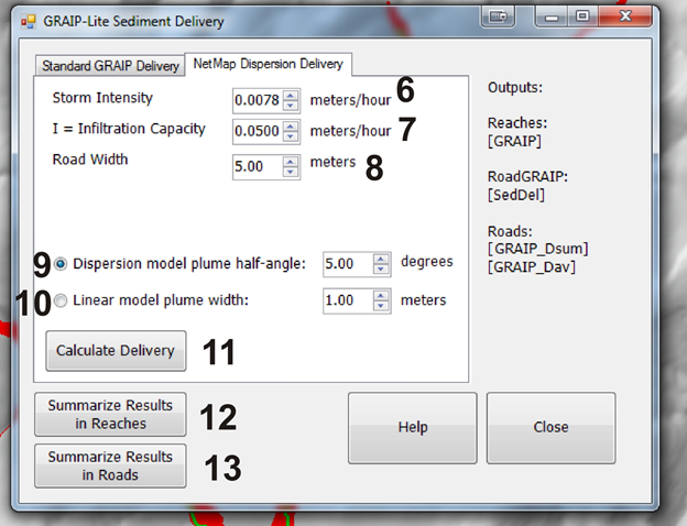 Figure 5. (8) in Figure 4 allows a user to select from two different sediment delivery models. (1) The standard GRAIP-Lite deliver method the uses the empirically derived relationship shown in Figure 3. The panel on the right shows the interface to implement NetMap's conservation of mass road sediment delivery model. Adjustable parameters include design storm intensity (6), steady state inflitration capacity (7), road width (8), the dispersion plume half angle (if selecting a triangular deposition plume) or a disperson plume width (10) if selecting a rectangular deposition plume. See Figure 6 for definitions and see more detailedi information on the Conservation of Mass Model. Once either the standard GRAIP-Lite model or NetMap's dispersion model is selected, results can be summarized to reaches (4), that is predicted road erosion sediment delivery can be mapped to the appropriate channel segments, and or (5) results can be summarized in the original road segment lengths (NetMap breaks roads into short segments for analysis, see NetMap's road drainage connectivity tool.
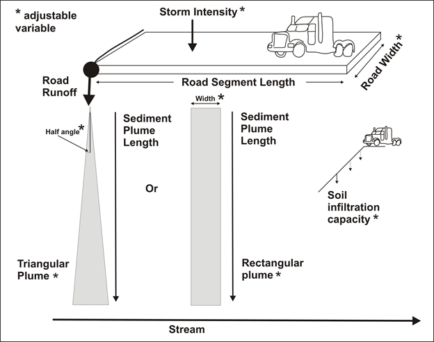 Figure 6. An illustration of the adjustable variables to run NetMap's conservation of mass road sediment delivery model (from Figure 5, right panel). To learn more about how this model was used in an analysis of road surface erosion, including getting credit for existing road erosion reduction programs, see short version or long version videos.
The eight types of output are shown below in Figures 7 through 13.
 Figure 7. GRAIP road sediment production, kg/yr, (in the GRAIP road layer). Delivery to streams is not considered.
 Figure 8. GRAIP road sediment production, kg/yr, delivered to streams (in the GRIAP road layer).
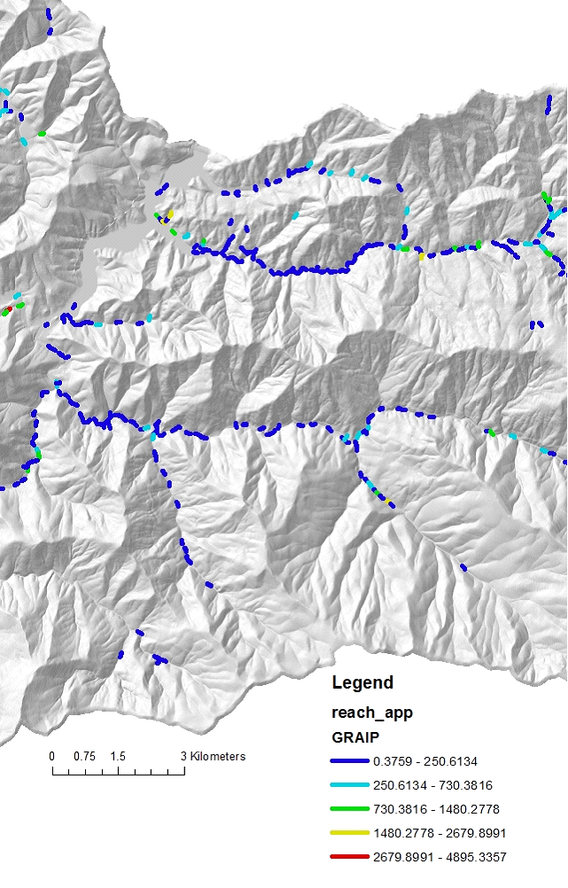 Figure 9. GRAIP road sediment production, kg/yr, delivered to streams (in the reach layer, per stream segment).
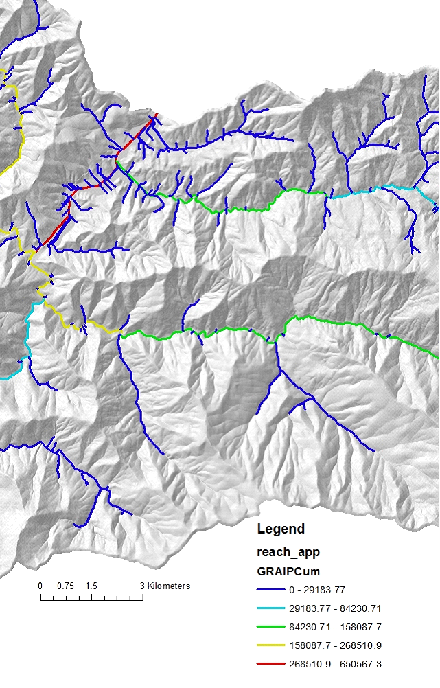 Figure 10. GRAIP road sediment production, kg/yr, delivered to streams and routed (area weighted) downstream (in the reach layer).
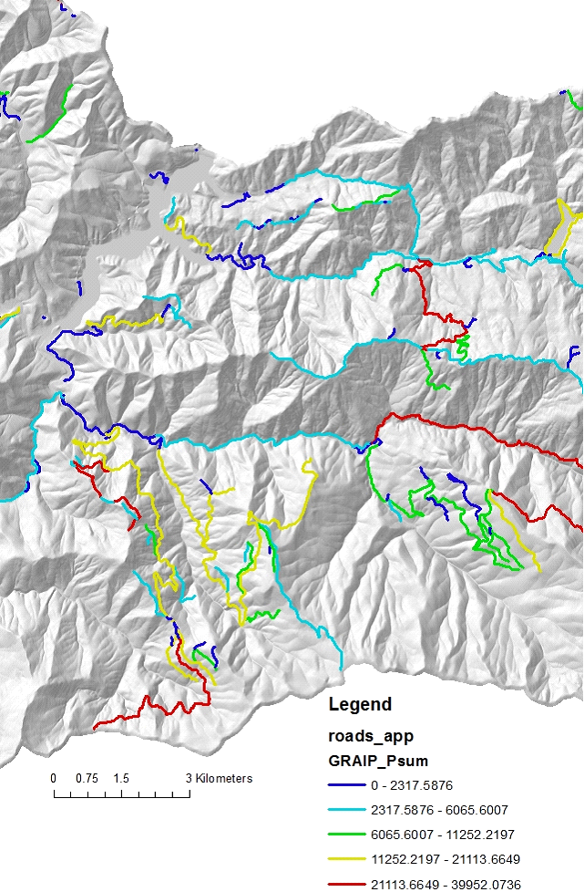 Figure 11. GRAIP road sediment production, summed in kg/yr, reported back to original road layer (referenced to unique road IDs).
 Figure 12. GRAIP road sediment delivery to streams, summed in kg/yr, reported back to original road layer (referenced to unique road IDs).
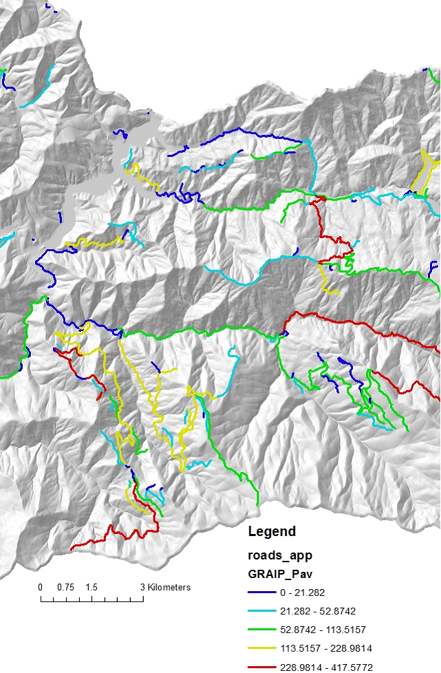 Figure 13. GRAIP road sediment production, length weighted in kg/yr/m, reported back to original road layer (referenced to unique road IDs).
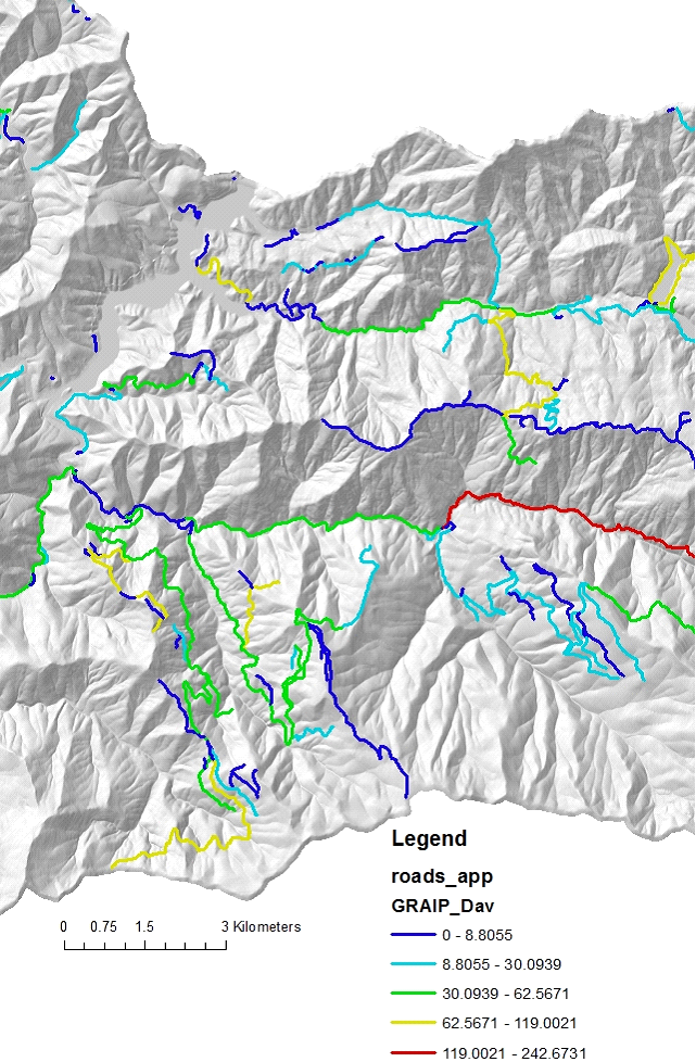 Figure 14. GRAIP road sediment delivery to streams, length weighted in kg/yr/m, reported back to original road layer (referenced to unique road IDs).
Interpretation
Care should be taken when interpreting GRAIP road erosion and sediment delivery predictions (similar to other erosion models). The prediction of road drain spacing (Figure 1) is only an approximation of the actual spacing that would be found in the field. Thus, the road erosion predictions made at that scale (i.e., a road segment scale of 100 m) do not reflect the reality of 100m road segments in the field (Figures 5 and 6). Thus it is best to consider road erosion and sediment delivery predictions at the scale of accumulated values of the original road segments (Figures 8 through 12). A similar caveat applies to sediment delivery predictions at the scale of individual channel segments (Figure 7).
Given this uncertainty, it is best to consider subbasin wide road erosion predictions that are characterized by downstream routed values (Figure 8). The routed stream values can be used to provide a general indication of which subbasins have roads that are at risk for sediment production (based on overall road length, road segment length [frequency of drainage structures], road slope, road surface type, road maintenance, and road proximity to streams). Once at risk subbasins have been identified, analysts can target those road networks for more intensive analyses, including full field based GRAIP analysis. In addition, NetMap’s Sort and Rank tool can be used to classify HUC 6th subbasins according to various GRAIP predictions.
Road erosion can be considered in context with impacts on aquatic systems, since road related erosion can negative impact fisheries (Everest et al. 1987, Luce et al. 2001). NetMap contains tools for predicting fish habitats. NetMap's overlap tool can be used to locate intersections of the highest road surface erosion potential with the best fish habitats.
Appendix 1:
Applying GRAIP as a Calibrated Road Impact Model
Charles Luce and Thomas Black May 29, 2012
The Geomorphic Roads Analysis and Inventory Package is designed with the intent to learn about the impacts of road systems on land surface processes and water. As the name implies it couples an inventory to analytical tools to build an approach to roads analysis that can be locally calibrated in a repeatable fashion with minimal effort. The full scope of GRAIP includes methods to inventory roads and analyze the inventory for surface erosion, gully risk, and landslide risk; methods to measure surface erosion from sample sites; and methods to estimate surface erosion where no inventory has been taken. The final part requires parameter estimates, which can be locally calibrated or, depending on required accuracy, assumed based on measurements in other areas. To date, manuals for inventory (Black et al., 2012) and reduction of inventory data (Cissel et al., 2012) have been completed, and a draft of the surface erosion measurement guide has been completed. Work is progressing on developing a prediction tool for areas outside of areas where inventories have been taken, and some insights from that work are provided here to illustrate the connections between inventory data, sediment collection data, and predictions. We begin with discussion of surface erosion modeling followed by discussion of sediment delivery and gully risk modeling.
Surface Erosion
Surface erosion has been modeled in the past with fairly simple empirical models, with more emphasis recently on so-called physically-based models. In any application of either empirical or physically based models, there is a need to define parameters to predict sediment. One of the promises of physically based models in contrast to empirical models is being able to define parameters that can work across many different precipitation regimes and soils. Values can then be identified for parameters that describe a range of soils such that they apply under whatever precipitation inputs might occur. The WEPP model is one such physically based model that has been applied to roads (e.g. Tysdal et al., 1999). The hydraulic conductivity is one of the key parameters in the WEPP model for predicting erosion (Tiscareno-Lopez et al., 1993), and substantial work was done with rainfall simulators and complex data analysis to find hydraulic conductivity for roads across a number of different soil textures (Luce and Cundy, 1994). Earlier work had been done to identify erodibility parameters for WEPP for a range of soil textures (Elliot et al., 1989).
The expectation for a physically based model is that parameters identified in this way could be applied over a range of climates and soils to predict erosion. Figure 1 shows the results of applying WEPP using soil texture and observed precipitation across a range of sites with measured soil erosion (Dubé et al., 2011). While there is somewhat of a general correspondence, the slope of the predicted erosion is somewhat flatter, and there is a slight tendency to overpredict. The Nash Sutcliffe of the WEPP predictions is 0.20 in normal space and -0.09 in log-transformed space, which would suggest that the mean observed erosion may serve better than the model to estimate erosion across this range of sites. Given that the range of erosion values spans 5 ½ orders of magnitude, that is not a particularly compelling case for trusting pre-calibration based on soil texture.
One likely reason for this result is that the hydrology of forest roads varies across sites based on interactions of soils and climate (Luce, 2002). In some places, particularly with tight soils and high precipitation intensity, hortonian overland flow (the hydrologic process modeled by WEPP) is common on roads (e.g. Ziegler, 2001), whereas in places with high conductivity soils (such as forests) and lower precipitation intensities or even snowmelt a greater proportion of road runoff is derived from cutslope interception (Burroughs et al., 1972; Megahan 1972, Wemple and Jones, 2003). For instance, at cutslopes in two different areas in Idaho Burroughs et al. (1972) and Megahan (1972) measured on the order of 95% of the runoff generated by cutslope interception. Note that the somewhat generally better performance for uncalibrated WEPP at sites in the southeastern US (Georgia, Tennessee, Oklahoma, Texas) compared to the sites in Oregon (Figure 1).
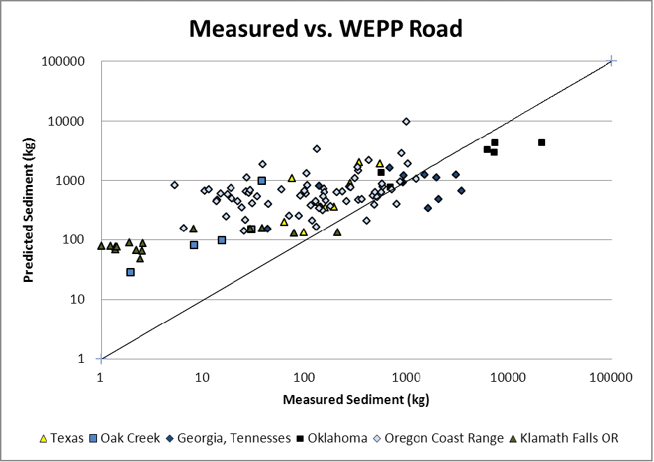 Figure 1: WEPP-Predicted versus observed surface erosion from 6 different road erosion experiments from Dubé et al. (2011). The Nash-Sutcliffe of the log-transformed results is -0.09.
By calibrating the WEPP model to better approximate the means for each group of sites, substantial improvements can be made (Figure 2). The Nash-Sutcliffe coefficient is 0.73 for untransformed and 0.61 for log-transformed data, which would rate the model as substantially useful with this mild degree of calibration. However, by taking this calibration step, WEPP functionally becomes an empirical model, raising the question of how WEPP predictions compare with empirical relationships. Tysdal et al. (1999) calibrated WEPP to road erosion data collected by Luce and Black (1999), and showed that similar patterns in erosion could be generated by the WEPP watershed model (but not the simpler plane-only version) and the segment length x slope ^2 regressions found by Luce and Black (1999). All plots experienced similar weather and had similar surfacing and ditch soil texture, so the WEPP model only used differences in slope and length. The GRAIP model uses a simpler Length x Slope model, which is easier to apply with less error in GIS. Comparison of predictions to observations of the calibrated GRAIP model show very similar performance to the calibrated WEPP model with Nash-Sutcliffe efficiencies of 0.72 and 0.60 for untransformed and log-transformed data respectively (Figure 3).
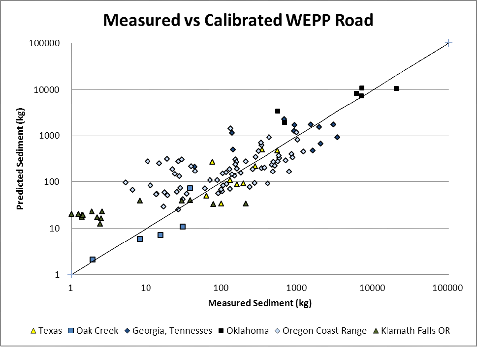 Figure 2: WEPP-Predicted versus observed surface erosion from 6 different road erosion experiments from Dubé et al. (2011) after calibrating WEPP to the mean erosion for each experimental group. The Nash-Sutcliffe of the log-transformed results is 0.61.
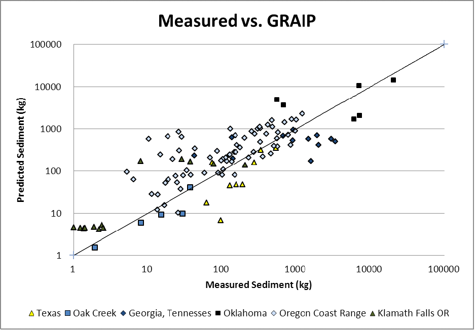 Figure 3: GRAIP-Predicted versus observed surface erosion from 6 different road erosion experiments from Dubé et al. (2011) after calibrating GRAIP to the mean erosion for each experimental group. The Nash-Sutcliffe of the log-transformed results is 0.60.
If all we can model in a given area is differences based on slope and contributing length, and if the effects of variations in soil texture and precipitation cannot be consistently reproduced by a physically based model, then it is valid to question whether the overhead of the multiple parameters in WEPP (the top 3 are hydraulic conductivity, rill erodibility, and interill erodibility) is acceptable, where the one parameter used by models like GRAIP or SedModl2 (a base rate) produces similar performance. While the virtues of model parsimony have been discussed in fairly academic terms and even quantified for model identification (e.g., Burnham and Anderson, 2002), the fundamental problem for applied usage comes in determining appropriate parameters.
The multiple parameters for the WEPP model can most reliably be found from rainfall simulation studies (e.g., Luce and Cundy, 1994), but those may not match whole-segment runoff and sediment generation characteristics due to mismatches in model physics and real physics, in which case a combination of runoff and sediment trap data can be used to fit parameters if some assumptions are used. In some circumstances, however, such data cannot be reasonably matched if the differences in physics are too great (e.g. Elliot et al., 1995). In contrast, the empirical models would just require the sediment trap data for calibration. While the empirical models would conceptually be poorer at modeling interannual variability due to precipitation variation, the examination of the uncalibrated WEPP model predictions would not support such a use of the WEPP model either. Again, if the physics are incorrect, only the rough general behaviors produced by road geometry that are similar regardless of runoff or erodibility parameters can be reliably reproduced. Further empirical analysis can be used to relatively easily determine relationships between sediment production and common BMPs such as gravel application (which varies locally in quality) or placing haul season or timing restrictions (e.g. Luce and Black 2001).
Having worked with the calibration of WEPP from both rainfall simulation data and sediment trap/flume data, and having worked with the validation of WEPP against observations for both calibrated and uncalibrated runs, we conclude that for practical purposes of applying measurements of erosion to inform erosion estimates from nearby road segments, simple models like GRAIP can be more reliable. Inventory data taken with the GRAIP model can be applied with empirical analysis of erosion plot data to generate as good of simulations as can be obtained from WEPP using similar calibration data, but at lower cost.
Sediment Delivery
One of the key aspects of road design and best management practice (BMP) application on Forest Roads is in the placement of roads and drainage features to minimize hydraulic connection between the roads and streams, promoting the infiltration of water into hillslopes and deposition of sediment. For this problem there is less tension between the potential for the physically based model and empirical models. It is generally well accepted that a Hortonian overland flow model should not be expected to reliably describe the hydrology of a forested hillslope except (potentially) under conditions of severe disturbance that limit the infiltration capacity of surface layers.
Delivery estimates by the WEPP model are essentially a function of the slope distance between the road and the stream. The actual functional relationship can be controlled through variation of the hydraulic conductivity parameter of the hillsllope. Validation of this kind of relationship can be done through visits to individual drain points and noting whether or not they connect to streams. Comparisons of two statistical models, one on slope distance (Figure 4), such as can be modeled using WEPP, and another on relative slope position (Figure 5), which further considers the distance from the ridge, show qualitatively similar results but a subtle difference in locations most near the stream, where the slope position metric shows a bit stronger probability. The Akaike Information Criterion (Burnham and Anderson, 2002) for the two models differ by more than 200, making the slope position model the much more likely model. WEPP also incorporates the amount of runoff from the road segment, which did not substantially improve predictions from the empirical analysis.
It is probably less important that the two different metrics performed differently in this case than to note that calibrating an empirical model of delivery versus simple topo-geomorphic metrics in an area is very straightforward using inventory data. Application of these empirical relationships in a predictive way for road segments that were not GRAIP inventoried is straightforward.
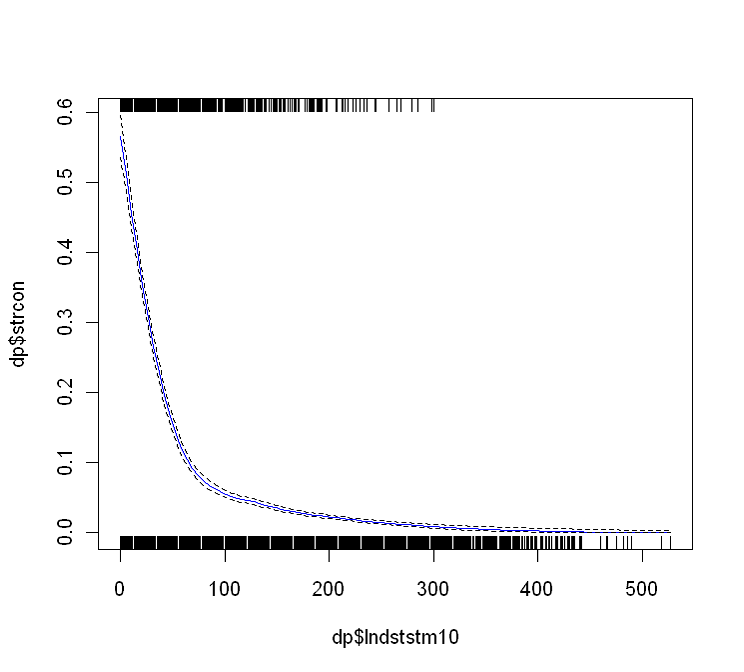 Figure 4. The linear distance to the stream (meters) for each drain point versus the probability of hydrologic connection to the channel at 13935 locations in southern Idaho. AIC=9485.
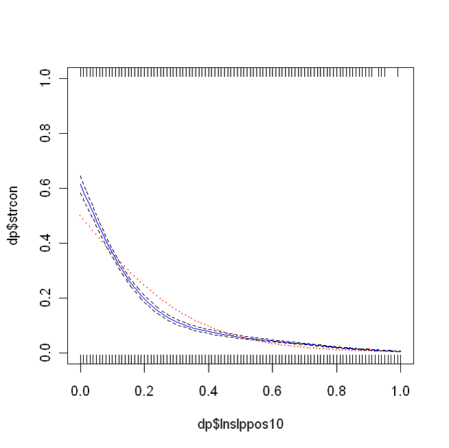 Figure 5. The slope position of a drain point versus the probability of hydrologic connection to the channel at 13935 locations in southern Idaho. The zero represents the stream and one represents the ridge top. The blue lines with black error bars is the local fit to the data, the red is a simple logistic regression fit. For the local logicstic fit, AIC = 9257.
Gullies
Substantial research has been done on gullies below roads (e.g. Croke and Mockler, 2001; Montgomery, 1994; Wemple et al., 1996). Many of these show unique relationships for the areas studied, and the areas that are studied tend to have a fairly high density of gullies below roads. It is after all difficult to study gullies in places where they are rare. For the general road manager, who may not have an interest in demonstrating a new theory on gullies, but who would like to use existing theory to determine how severe issues are locally and explore what would be necessary to control it. By collecting data along a series of road segments using the GRAIP protocol, information can be generated to allow creating plots like those in figure 6 that can show locally derived relationships between the length of the contributing road segment, the slope of the hill it puts water onto, and the likelihood that a gully will be generated. If the process were a simple threshold as has been generally suggested, there would be a step from 0 probability to 1 probability at some ESI value. The varying slopes as ESI increases are due to spatial variations in the strength of the soil due to soil characteristics and rooting strength. Gully probability can be controlled by managing the length of road segment leading to each drain point and directing drainage to lower slope areas, or taking water in ditches all the way to road-stream crossings (which increases runoff and sediment connectivity).
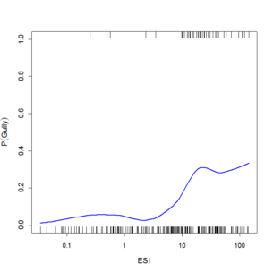 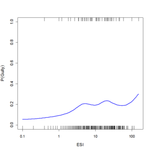 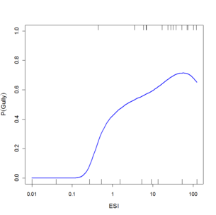 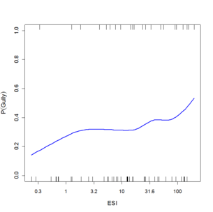 Figure 6: Plots of gully probability as a function of ESI (segment length times the square of the slope of the receiving hillside) for roads near a) South Fork Payette River near Lowman, b) South Fork Skokomish River, c) Pierce-Prairie Road near SF Boise R., and d) Skykomish R. derived from local logistic regression of observations across several culverts. Substantial variability is seen in both the degree of risk as ESI becomes high and in how it trends from low values to high. The tick marks on the inside of the upper and lower axes are observed gullies and non-gullies respectively, and the blue line is the fit between them showing the probability of a gully for that value of ESI.
Summary
The discussion here is about the evolution of road erosion modeling approaches to be more responsive to local data, information, and experience in a way that can be quantified. Philosophically the approach grows out of the idea that while approximate models are useful and adequate in many areas, when the stakes are high and managers need to reduce uncertainty among a variety of stakeholders, an efficient means is needed to collect and apply data to reduce model uncertainty. The conceptually simple empirical relationships employed in the approach can be updated as we learn more about road runoff and erosion processes more generally.
Empirical relationships like these can be very easily applied in GIS based models. The full GRAIP model can display these characteristics where a full inventory has been completed. Work is progressing on a model for prediction where roads are not fully inventoried.
References
Black, T. A., Cissel, R. M., Luce, C. 2012. The Geomorphic Roads Analysis and Inventory Package (GRAIP) Volume 1: data collection method. RMRS-GTR-280. USDA Forest Service, Rocky Mountain Research Station, Boise, ID. 115 pp.
Burnham, K. P., and D. R. Anderson (2002), Model Selection and Multimodel Inference, 2nd ed., 488 pp. Springer, New York.
Burroughs Jr ER, Marsden MA, Haupt HF. 1972. Volume of snowmelt intercepted by logging roads. Journal of Irrigation and Drainage Division ASCE 98: 1–12.
Cissel, R., Black, T., Schreuders, K. A. T., Prasad, A., Luce, C., Tarboton, D. G., Nelson, N. 2012. The Geomorphic Roads Analysis and Inventory Package (GRAIP) Volume 2:Office Procedures. RMRS-GTR-281. US Department of Agriculture, Forest Service, Rocky Mountain Research Station, Boise, ID. 162 pp
Croke J, Mockler S. 2001. Gully initiation and road-to-stream linkage in a forested catchment, southeastern Australia. Earth Surface Processes and Landforms 26: 205–217.
Dubé, K., T. Black, C. Luce, and M. Riedel, 2011, Comparison of Road Surface Erosion Models with Measured Road Surface Erosion Rates. Technical Bulletin No. 0988. National Council for Air and Stream Improvement, Inc. Research Triangle Park, NC.
Elliot, W.J., C.H. Luce, and P.R. Robichaud, 1996, Predicting Sedimentation from Timber Harvest Areas with the WEPP Model, Proceedings of the Sixth Interagency Sedimentation Conference, March 10-14, 1996, Las Vegas, NV. pp. IX:46-53.
Elliot, W.J.; Liebenow, A.M.; Laflen, J.M.; Kohl, K.D. 1989. A Compendium of Soil Erodibility Data from WEPP Cropland Soil Field Erodibility Experiments 1987 and 1988. NSERL Report No. 3, The Ohio State University, and USDA Agricultural Research Service
Luce, C. H. and T. W. Cundy, 1994, Parameter identification for a runoff model for forest roads, Water Resources Research, 30(4):1057-1069.
Luce, C.H. and T.A. Black, 1999, Sediment production from forest roads in western Oregon. Water Resources Research 35(8):2561-2570.
Luce, C.H. and T.A. Black 2001, Effects of Traffic and Ditch Maintenance on Forest Road Sediment Production, In Proceedings of the Seventh Federal Interagency Sedimentation Conference, March 25-29, 2001, Reno, Nevada. pp. V67–V74.
Luce, C. H. 2002, Hydrological Processes and Pathways Affected by Forest Roads: What Do We Still Need to Learn?, Hydrological Processes, 16, 2901-2904.
Megahan WF. 1972. Subsurface flow interception by a logging road in mountains of central Idaho. In Proceedings, National Symposium on Watersheds in Transition. American Water Resources Association: Fort Collins, CO; 350–356.
Montgomery DR. 1994. Road surface drainage, channel initiation, and slope instability. Water Resources Research 30:1925–1932.
Tiscareno-Lopez, M., Lopes, V. L., Stone, J. J. and Lane, L. J. 1993, Sensitivity analysis of the WEPP watershed model for rangeland applications I: Hillslope component. Trans. ASAE 36, 1659-1672.
Tysdal, L.M., W.J. Elliot, C.H. Luce, and T.A. Black. 1999. Modeling Erosion from Insloping Low-Volume Roads with WEPP Watershed Model. Transportation Research Record, 1652:250-256.
Wemple BC, Jones JA, Grant GE. 1996. Channel network extension by logging roads in two basins, western Cascades, Oregon. Water Resources Bulletin 32: 1195–1207.
Wemple, B.C. and J.A. Jones. 2003. Runoff production on forest roads in a steep, mountain catchment. Water Resources Research 39, doi:10.1029/2002WR001744.
Ziegler AD, Giambelluca TW, Sutherland RA, Vana TT, Nullet, MA. 2001. Horton overland flow contribution to runoff on unpaved mountain roads: a case study in northern Thailand. Hydrological Processes 15: 3203–3208.
|